Implementing General Relativity: Rendering the Schwarzschild black hole, in C++
General relativity is pretty cool. Doing anything practical with it is a bit of a pain, and a lot of information is left to the dark arts. More than that, a significant proportion of information available on the internet is unfortunately incorrect, and many visualisations of black holes are wrong in one way or another - even ones produced by physicists! We’re going to focus on two things:
- Giving you a practical crash course in the theory of general relativity
- Turning this into code that actually does useful things
This tutorial series is not going to be a rigorous introduction to the theory of general relativity. There’s a lot of that floating around - what we’re really missing is how to translate all that theory into action
By the end of this infinitely long tutorial series, you will smash black holes and neutron stars together, without a supercomputer, in just a few minutes flat 1
Our first step along this journey is the classic starting point: The schwarzschild black hole
What are we actually simulating?
The end goal here is to end up with this:
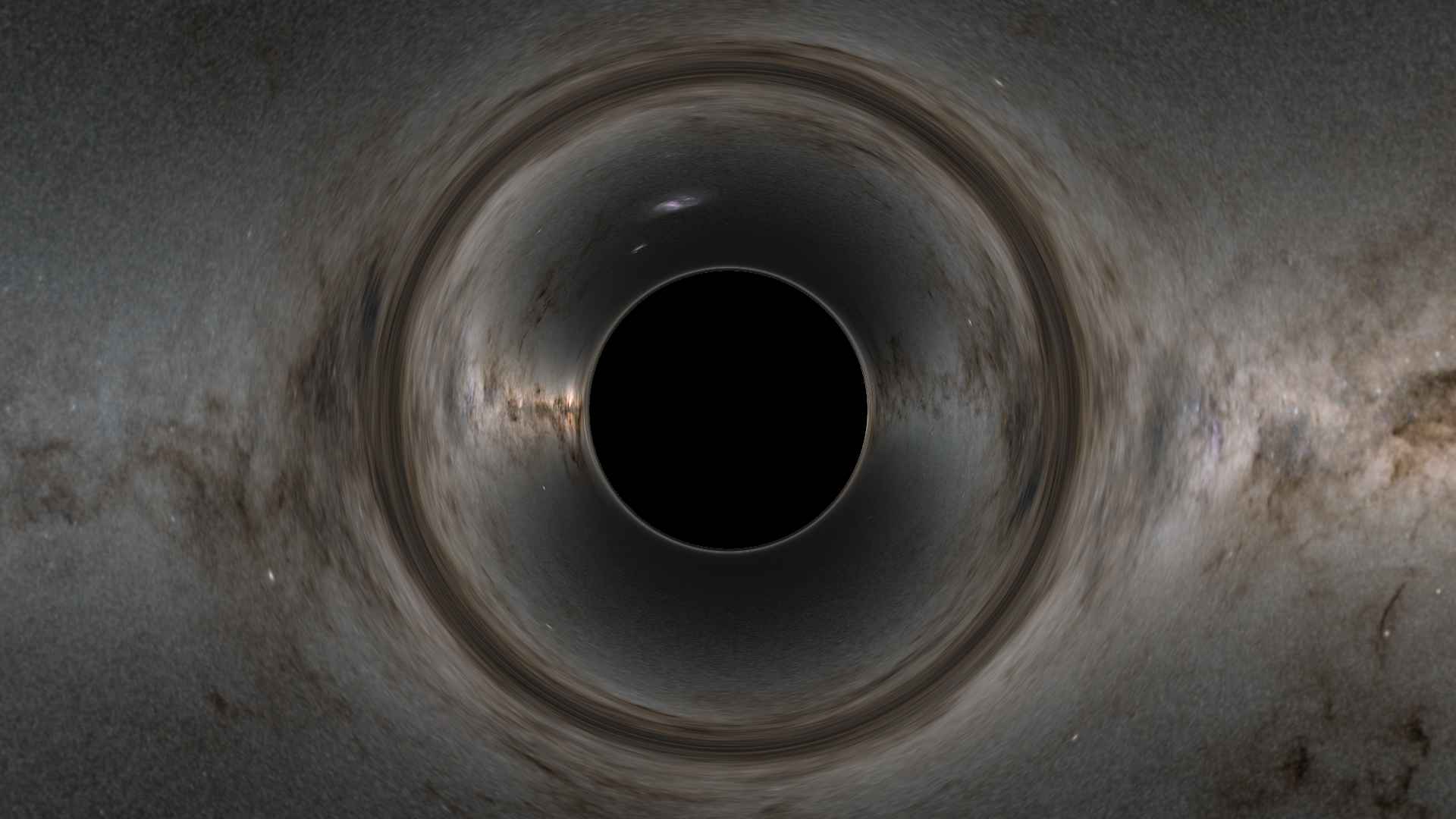
First up, a black hole isn’t a physical thing you can touch, and the schwarzschild black hole isn’t made of anything tangible. It exists purely gravitationally - its a stable, self supporting gravitational field. It is made up of spacetime being curved, and nothing else. The schwarzschild black hole is in the class of objects known as a “vacuum solution”, which is to say that there is no matter or what you might call mass2 present whatsoever
What we actually see in this picture is purely as a result of spacetime being curved, bending the path of anything that travels through it. We create light rays at the camera, trace them around our curved spacetime according to the equations of general relativity, and then render the background according to where our rays of light end up. Some rays of light get trapped at the event horizon, resulting in the black ‘shadow’ of the black hole
There’s a reason I got into programming and not art
Breaking down a simulation
There are 3 parts to any simulation
- The initial conditions
- The evolution equations
- Termination
We’re going to be focusing on the pipeline of simulating this from start to end, with complete examples so that nothing gets left in the gaps
Step 1 will be left until last, and is not the focus of this article. Step 2 requires us to solve something called the geodesic equation: which is the equation of motion for a ray of light (and objects in general) in general relativity. To be able understand it we’ll need some background
Mathematical background
Tensor index notation
General relativity uses its own specific conventions for a lot of maths that is somewhat dense at first glance, though very expressive once you get used to it. There’s one key idea compared to maths you might be more familiar with, that we need to get a handle on first before we go anywhere else today:
Contravariance, and covariance
In everyday maths, a vector is just a vector. We informally express this as something like $v = (1,2,3)$ or $v = 1x + 2y + 3z$, where $x$ $y$ and $z$ are our coordinate system basis vectors3. When dealing with vectors, its common to index the vector’s components by an index as a shorthand:
\[\sum_{k=0}^2 v_k == v_0 + v_1 + v_2\]This is an example of how we’d express summing the components of a vector. Tensor index notation takes this notation one step further, by giving the vertical positioning of the index (here $_k$ ) additional meaning. In general relativity, $v_k$, and $v^k$ mean two different things. Indices can be:
Objects such as matrices have more than one index, and the indices can have any “valence” (up/down-ness). For example, $A^{\mu\nu} $, $ A^\mu_{\;\;\nu} $, $ A_\mu^{\;\;\nu} $, and $ A_{\mu\nu} $ are all different representations of the same object $A$. The first is the contravariant form, the middle two have mixed indices, and the last one is the covariant form. We can add more dimensions to our objects too: eg: $ \Gamma^\mu_{\;\;\nu\sigma} $5 is a 4x4x4 object here. Here I will call all of these objects ‘tensors’6
The physical interpretation of this, and what it really means for an index to be contravariant or covariant is difficult to interpret unfortunately, so this section is going to feel very arbitrary. This is one of those things you’ll just have to roll with, until you’re a lot deeper into the maths
One thing to note: Tensors and scalars (objects without indices) are generally functions of the coordinate system, and vary from point to point in our spacetime. While we write $A_{\mu\nu}$, what we really mean is $A_{\mu\nu}(x, y, z, w)$ - its secretly a function that returns a 4x4 matrix, when we feed coordinates into it
Raising and lowering indices
The most important object in general relativity is the metric tensor, spelt $g_{\mu\nu}$, and it is generally given in its covariant form. This object defines spacetime - how it curves, how we measure lengths and angles - and virtually everything in general relativity involves the metric tensor in some form or other
The metric tensor is a 4x4 symmetric matrix. Because it is symmetric, $ g_{\mu\nu} = g_{\nu\mu} $, and as a result only has 10 independent components. The metric tensor is also often thought of as a function taking two arguments, $g(u,v)$, and performs the same role as the euclidian dot product. That is to say, where in 3 dimensions you might say $a = dot(v, u)$, in general relativity you might say $a = g(v, u)$
For the metric tensor, and the metric tensor only, the contravariant form of the metric tensor is calculated as such:
\[g^{\mu\nu} = (g_{\mu\nu})^{-1}\]Ie, the regular 4x4 matrix inverse of treating $g$ as a matrix7
The metric tensor is responsible for many things, and one of its responsibilities is raising and lowering indices. To raise an index, we do it as such:
\[v^\mu = g^{\mu\nu} v_\nu\]And lowering an index is performed like this:
\[v_\mu = g_{\mu\nu} v^\nu\]I’ve introduced some new syntax here known as the einstein summation convention, so lets go through it. In general, any repeated index (a ‘dummy’ index) in an expression is summed:
\[g_{\mu\nu} v^\nu == \sum_{\nu=0}^3 g_{\mu\nu} * v^\nu\]with $*$ being normal scalar multiplication, which is always unwritten. In code, this looks like this, which may be clearer:
tensor<float, 4> lower_index(const tensor<float, 4, 4>& metric, const tensor<float, 4>& v) {
    tensor<float, 4> result = {};

    //mu is a free index
    for(int mu = 0; mu < 4; mu++) {
        float sum = 0;
        //nu is a dummy index
        for(int nu = 0; nu < 4; nu++) {
            sum += metric[mu, nu] * v[nu];
        }
        result[mu] = sum;
    }

    return result;
}
A more complicated expression looks like this:
\[\Gamma^\mu_{\nu\sigma} v^\nu u^\sigma == \sum_{\nu=0}^3 \sum_{\sigma=0}^3 \Gamma^\mu_{\nu\sigma} v^\nu u^\sigma\]tensor<float, 4> example(const tensor<value, 4, 4, 4>& christoff2, const tensor<value, 4>& v, const tensor<value, 4>) {
tensor<float, 4> result = {};
//mu is a free index
for(int mu = 0; mu < 4; mu++) {
float sum = 0;
//nu is a dummy index
for(int nu=0; nu < 4; nu++) {
//sigma is a dummy index
for(int sigma = 0; sigma < 4; sigma++) {
sum += christoff2[mu, nu, sigma] * v[nu] * u[sigma];
}
}
result[mu] = sum;
}
return result;
}
Here, $\nu$ and $\sigma$ are ‘dummy’ indices (ie they are repeated), and $\mu$ is a ‘free’ index (not repeated). Each dummy index is summed only with itself, and they form the bounds for our $\sum_{}$’s
The size of the resulting tensor is equal to the number of free indices. One more rule is that only indices of opposite valence sum: eg an up index only sums with a down index, and you do not sum two indices of the same valence - though this almost never crops up. Jump to the indices footnote for more examples
Raising and lowering multidimensional objects
The last thing we need to learn now is how to raise and lower the indices of a multidimensional object, eg $ A^{\mu\nu} $. To do this, you set a dummy index to the slot we wish to change the valence of - lets say the second, giving $A^{\mu i}$. Then, the metric tensor gets the dummy index in one slot giving $g_{i ?}$, and the original free index in the other slot giving $g_{i\nu}$. The full expression is then: $g_{i\nu} A^{\mu i} = A^{\mu}_{\;\;\nu}$. The contravariant form of the metric tensor is used to raise indices, and the covariant form is used to lower them
More examples are provided in the indices footnote
If like me you’ve hit this point and are feeling a bit tired, don’t worry. These are rules we can refer back to whenever we need them, and the footnotes will contain lots of examples. Here’s a picture of my cat for making it this far:

Raytracing as differential equations, in 3d
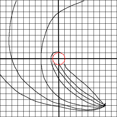
What we’re trying to accomplish here in this article is basic raytracing. In a normal, 3d raytracer, we construct a ray with a start position $x^i$, and a velocity $v^i == \frac{dx^i}{ds}$, where $s$ is a parameter that is often time. If we’re raytracing simple 3d graphics, rays travel in straight lines. In general, we don’t care about the magnitude of $v^i$, as it simply corresponds to rescaling $ds$. Eg 3 meters/second is equivalent to 30 meters/decasecond
Lets imagine that our rays do not move in straight lines, and that at every point in space, an acceleration $a^\mu$ is applied to our ray. To find the points on our ray in the general case, we must integrate some basic equations of motion. That is to say, we need to solve the following equations for $x$
\[\begin{align} \frac{dx^\mu}{ds} &= v^\mu \\ \\ \frac{dv^\mu}{ds} &= a^\mu\\ \end{align}\]In newtonian dynamics, $a^\mu$ might be the acceleration given by all the other bodies in our simulation applying a force to us (which we will label with the index ${m}$):8
\[a^\mu = (-G \sum_{k=0, k != m}^n \frac{m_k}{|x_m - x_k|^3} (x_m - x_k))^\mu\]And in straight line raytracing, $a^\mu=0$, allowing us to directly integrate the equations
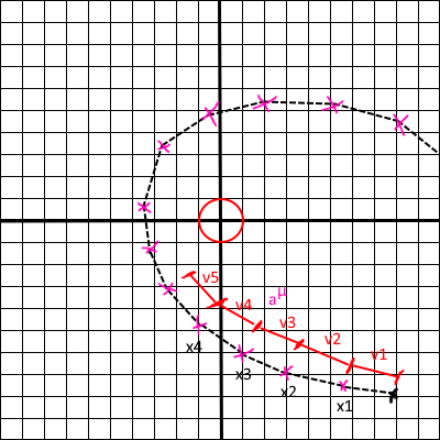
Here, each $x$ is a point along the integrated curve, $v$ is a velocity multiplied by our timestep (which is the segment length in euler integration), and the purple checkmarks $a^\mu$ are where we evaluate the acceleration
Geodesics
Geodesics: the basics
In general relativity:
\[a^\mu = -\Gamma^\mu_{\alpha\beta} v^\alpha v^\beta\]Where $\Gamma^\mu_{\alpha\beta}$ is derived from the metric tensor, and is implicitly a function of $x^\mu$. This is called the geodesic equation9, and describes the motion of GR’s notion of rays, which are called geodesics - these are curves through our coordinate system
In general relativity, the motion of all objects and lightrays are described by geodesics. On earth, if you move in a straight line you’ll end up going in a circle: geodesics are the more mathematical version of this concept. The only physically accurate way to get from point A, to point B, or relate them in any fashion in the general case, is via a geodesic
Timelike, lightlike, and spacelike geodesics
There are three kinds of geodesics:
- Timelike: these are paths which can be travelled by an observer (or particle) with mass (even if very minimal)
- Lightlike: these are paths which can only be travelled by light10
- Spacelike: these geodesics are a bit more complicated to interpret, and we will ignore them. They represent paths that are causally disconnected from us
The metric tensor defines which one of these categories a geodesic falls into, depending on its velocity $v^\mu$
- Timelike: $g_{\mu\nu} v^\mu v^\nu < 0$
- Lightlike: $g_{\mu\nu} v^\mu v^\nu = 0$
- Spacelike: $g_{\mu\nu} v^\mu v^\nu > 0$
Note that there are alternate definitions11. Geodesics cannot change their type, so a timelike geodesic is timelike everywhere along the curve it traces out
We’d like to render our black hole by firing light rays around and finding out what our spacetime looks like, so what we’re looking for in this article is lightlike geodesics, where $g_{\mu\nu} v^\mu v^\nu = 0$
Geodesics: the less basics
A geodesic has two properties: a position $x^\mu$, and a velocity $v^\mu$. Velocity is defined as the rate of change of position $dx^\mu$ with respect to some parameter $ds$, giving $\frac{dx^\mu}{ds}$. We have a choice of several parameters we could use:
- The concept of time given to us by our coordinate system, which is completely arbitrary and has no meaning, often called $dt$
- The concept of time as experienced by an observer (including particles), called proper time, $d\tau$
- A fairly arbitrary parameter called $ds$, that simply represents how far we’re moving along our curve
No observer can move at the speed of light, so 2. is right out for lightlike geodesics, though works well for timelike geodesics. 1. Is dependent on our coordinate system and is hard to apply generally (not every coordinate system has a time coordinate), and we have to modify our geodesic equation as well. So in general, we will always be using 3 for light
This makes our velocity: $v^\mu = \frac{dx^\mu}{ds}$ - which we already knew, but now we know what $ds$ means - which in this case is not all that much. The specific $ds$ we get from case 3. is known as an affine parameter, and represents a parameterisation of our curve/geodesic. The geodesic equation that we have already seen is adapted for this parameterisation12
Integrating the geodesic equation
We’re going to solve one of our major components now: We’ve already briefly seen the geodesic equation9, which looks like this:
\[a^\mu = -\Gamma^\mu_{\alpha\beta} v^\alpha v^\beta\]Where more formally, our acceleration $ a^\mu = \frac{d^2x^\mu}{ds^2} $, $v^\mu = \frac{dx^\mu}{ds}$, and
\[\Gamma^\mu_{\alpha\beta} = \frac{1}{2} g^{\mu\sigma} (g_{\sigma\alpha,\beta} + g_{\sigma\beta,\alpha} - g_{\alpha\beta,\sigma})\]is how we calculate $\Gamma^\mu_{\alpha\beta}$, an object known by the catchy name “christoffel symbols of the second kind”13. Note that:
\[g_{\mu\nu,\sigma} == \partial_\sigma g_{\mu\nu}\]Ie, taking the partial derivatives in the direction $\sigma$, as defined by our coordinate system. This equation is likely to stretch our earlier understanding of how to sum things, so we’ll write it out manually14:
\[\Gamma^\mu_{\alpha\beta} = \frac{1}{2} \sum_{\sigma=0}^3 g^{\mu\sigma} (\partial_\beta g_{\sigma\alpha} + \partial_\alpha g_{\sigma\beta} - \partial_\sigma g_{\alpha\beta})\]or
tensor<float, 4, 4, 4> Gamma;

for(int mu = 0; mu < 4, mu++)
{
    for(int al = 0; al < 4; al++)
    {
        for(int be = 0; be < 4; be++)
        {
            float sum = 0;

            for(int sigma = 0; sigma < 4; sigma++)
            {
                sum += 0.5f * metric_inverse[mu, sigma] * (diff(metric[sigma, al], be) + diff(metric[sigma, be], al) - diff(metric[al, be], sigma));
            }

            Gamma[mu, al, be] = sum;
        }
    }
}
Phew. This loop may look quite slow to calculate, and it is. GR is not cheap to render in the general case. There are some symmetries here that reduce the computational complexity, notably that $\Gamma^\mu_{\alpha\beta} = \Gamma^\mu_{\beta\alpha}$, $g_{\mu\nu} = g_{\nu\mu}$, and $g^{\mu\nu} = g^{\nu\mu}$. Additionally, in many metrics most of $\Gamma$’s components are 0, which helps too
So: to integrate a geodesic, we start off with an appropriate position, $x^\mu$, an appropriate velocity, $v^\mu$, and calculate our acceleration via the geodesic equation. We then integrate this. During the process of this, we’ll need a metric tensor $g_{\mu\nu}$ and the partial derivatives of it
We’re getting close to being able to integrate our equations now. We now need three more things:
- A real metric tensor
- An initial position $x^\mu$, which will be our camera position
- An initial velocity, which is more complex
A real metric tensor
There are many different black holes, and many different ways of representing each of them. Today we’re going to pick the simplest kind: the schwarzschild black hole - a black hole with only a mass parameter, and no charge or spin. A spacetime like schwarzschild is defined by its metric tensor, and this is often expressed in a form called the “line element”:
\[ds^2 = -d\tau^2 = -(1-\frac{r_s}{r}) dt^2 + (1-\frac{r_s}{r})^{-1} dr^2 + r^2 d\Omega^2\]This is the wikipedia definition15, where $d\Omega^2 = d\theta^2 + sin^2(\theta) d\phi^2$, and $r_s$ is the schwarzschild radius - that is twice the ‘mass’2 $M$ in geometric units of $c=g=1$. This equation completely defines the schwarzschild spacetime, and the black hole within it
Lets examine this in more detail. The $d$ terms on the right hand side (eg $dt$) represent infinitesimals. $ds^2$ is called the spacetime interval: note that it can be negative, or 0. The fact that this $ds^2$ and the $ds$ we picked for our parameterisation are the same is not a total coincidence - for timelike curves, we generally pick $ds_{parameterisation} = d\tau$. In reality, $ds$ refers to the general concept of arc length, which is why the notation is re-used
The sign15 of $ds^2$ defines what kind of geodesic we have. If we plug a velocity $(dt, dr, d\theta, d\phi)^\mu = v^\mu$ in here, and calculate the metric at our position $(t, r, \theta, \phi)^\mu = x^\mu$, then:
- If $ds^2 > 0$, our curve is spacelike
- If $ds^2 == 0$, our curve is lightlike, and is the path light takes
- If $ds^2 < 0$, our curve is timelike, and is the path an observer takes
This is strictly equivalent to our earlier set of definitions, where we simply used the metric in matrix form. Note that $d\tau$ only takes on a value if $ds^2 <= 0$ - but it is only actually valid due to how it is derived if $ds^2 < 0$. This is a more mathematical way of saying that only a timelike curve - the path that an observer takes - has a definition of proper time. This makes sense, because proper time is the time experienced by an observer
$ds^2$ is invariant. No matter who plugs in their own values for some $v^\mu$ into our line element, if its the same object, even though different observers might disagree on the values of $v^\mu$, everyone will agree on $ds^2$
Reading the metric tensor from the line element
We can read the matrix $g_{\mu\nu}$ directly off from the line element16. If we have the line element (with the displacement $(d_0, d_1, d_2, d_3)$)
\[ds^2 = k_1 d_0^2 + k_2 d_0d_1 + k_3 d_0d_2 + k_4 d_0d_3 + k_5 d_1^2 + k_6 d_1 d_2 + k_7 d_1 d_3 + k_8 d_2^2 + k_9 d_2 d_3 + d_{10} d_3^2\]We get the metric tensor $g_{\mu\nu}$:
| . | $d_0$ | $d_1$ | $d_2$ | $d_3$ |
|---|---|---|---|---|
| $d_0$ | $k_1$ | $\frac{1}{2} k_2$ | $\frac{1}{2} k_3$ | $\frac{1}{2}k_4$ |
| $d_1$ | $\frac{1}{2}k_2$ | $k_5$ | $\frac{1}{2}k_6$ | $\frac{1}{2}k_7$ |
| $d_2$ | $\frac{1}{2} k_3$ | $\frac{1}{2}k_6$ | $k_8$ | $\frac{1}{2}k_9$ |
| $d_3$ | $\frac{1}{2}k_4$ | $\frac{1}{2}k_7$ | $\frac{1}{2}k_9$ | $k_{10}$ |
Being triply clear, this means that eg $g_{00} == k_1$, and $g_{20} == \frac{1}{2} k_3$. Note that all offdiagonal terms are multiplied by $\frac{1}{2}$. In the schwarzschild case, we get:
| . | t | r | $\theta$ | $\phi$ |
|---|---|---|---|---|
| t | $-(1-\frac{r_s}{r})$ | 0 | 0 | 0 |
| r | 0 | $(1-\frac{r_s}{r})^{-1}$ | 0 | 0 |
| $\theta$ | 0 | 0 | $r^2$ | 0 |
| $\phi$ | 0 | 0 | 0 | $r^2 sin^2(\theta)$ |
Remember that this matrix is a function of the coordinate system, and it must be recalculated at a specific point in space where you want to use it. If you want to raise or lower the velocity of a geodesic, you must calculate the metric tensor at the position where the velocity vector is, ie $x^\mu$17
While you can evaluate whether or not a geodesic is timelike, or lightlike by using the line element - you can also directly use the metric tensor in its matrix form, as such:
\[ds^2 = -d\tau^2 = g_{\mu\nu} v^\mu v^\nu\]Numerical differentiation vs automatic differentiation
Now that we have our metric tensor, we need to take its derivatives. There are two easy ways to calculate the derivatives: numerical differentiation, and automatic differentiation. A post I made recently covered AD, and I would recommend using it. However here, we will approximately define the derivatives for space savings. Remember that the metric tensor is calculated at a coordinate, and is a function of the coordinate system. Lets make this explicit, by defining $g_{\mu\nu}$ as $g_{\mu\nu}(t, r, \theta, \phi)$
\[g_{\mu\nu,t} = \partial_t g_{\mu\nu} == \frac{(g_{\mu\nu}(t + h, r, \theta, \phi) - g_{\mu\nu}(t - h, r, \theta, \phi))}{2h}\]This is a simple centered derivative to calculate the derivative in the first coordinate direction, often called $\partial_0$, which is equivalent to $\partial_t$ in schwarzschild
A brief pause to review
So far we have:
-
Defined the paths that lightrays take as likelight geodesics. These have a position $x^\mu$, and a velocity $v^\mu$. We know these are geodesics where $g_{\mu\nu} v^\mu v^\nu = 0$
-
Found out how to read a metric tensor $g_{\mu\nu}$ from a line element
-
Understood how to plug numbers into the geodesic equation, to get our acceleration
It might surprise you to learn that this is the simple part of what we’re trying to do, in general. For the purposes of trying to minimise the sheer information overload today before we get up and running with our first black hole, I’m going to present some pre-baked initial conditions, instead of calculating them the long way round
Initial conditions
Initial conditions in this corner of general relativity are not a good, fun time. This is where we get into the less well understood corners of general relativity, and where mistakes tend to be made. We’re going to condense a much longer future discussion of initial conditions into a future article in this series - likely when you all conveniently go on holiday
What are we trying to get out of our initial conditions?
In this phase, what we’re trying to do is construct an initial geodesic velocity $v^\mu$ that represents where our lightray is going. In a regular, flat, 3d simulation, its very easy - you define a plane in front of the camera, and construct a ray, from the camera’s origin, through a pixel on that plane. If a pixel has a position $p=(x-width/2, y-height/2, f)$ (f being the planes distance from the camera) on that plane, then the ray’s direction in 3d space is $d=norm(p)$
The question then becomes: how do we translate that ray direction $d$ in 3d space, to a valid geodesic velocity in 4d spacetime? The answer is: tetrads
Tetrads are the 10th circle of hell
Tetrads, also known as frame fields, or vielbein, are a field of four 4-vectors, that are orthonormal (ie perpendicular, and unit lengthed, with respect to the metric tensor). These make up the “frame of reference” of an observer, and are used to translate between what one observer sees and experiences, and the wider universe that we’re describing
General relativity demands that spacetime is locally flat from the perspective of any observer. And yet, we can observe that spacetime is clearly curved - planets go round the sun, and black holes exist. Translating from an observers locally flat spacetime, to that curved spacetime, is done via our tetrads. These are the objects that define the disconnect between “my space is locally flat” and “my friends space is clearly curved”, and also how you translate observations between two different observers
Tetrads are basis vectors, for pushing vectors from an observers locally flat space, to our curved spacetime. Each tetrad vector is labelled with a latin index $i$, and are given by $e_i$. Each one of these tetrad vectors $e_i$ has 4 components, and so they are spelt $e^\mu_i$ in the literature with stacked indices. This makes up a 4x4 matrix when treated as column vectors, and the inverse (which is a matrix inverse $(e^\mu_i)^{-1}$) is spelt $e_\mu^i$. If this seems needlessly extremely confusing, you are absolutely correct horse. Some papers18 use $\theta_\mu^i$ to denote the inverse
Note that when dealing with tetrads, latin indices $i,j,k$ refer to ‘local’ quantities in your flat spacetime, and greek indices $\mu,\nu,\sigma$ refer to quantities in your coordinate space
Spacetime is locally flat
The technical definition of locally flat is the minkowski metric, $\eta_{ij}$, which is always in cartesian coordinates + time, no matter the coordinate system of our metric tensor $g_{\mu\nu}$:
| t | x | y | z | |
|---|---|---|---|---|
| t | -1 | 0 | 0 | 0 |
| x | 0 | 1 | 0 | 0 |
| y | 0 | 0 | 1 | 0 |
| z | 0 | 0 | 0 | 1 |
Or as a line element, $ds^2 = -d\tau^2 = -dt^2 + dx^2 + dy^2 + dz^2$
Here we want to make a light ray, which is defined as such:
\[v_{flat}^i = (1, d_0, d_1, d_2)\]Where $ \lvert d \rvert = 1 $.
Note that $\eta_{ij} v^i_{flat} v^j_{flat} = 0$, which makes this a lightlike geodesic in our minkowski spacetime19
Each tetrad defines a series of basis vectors which we can use to transform from our flat minkowski spacetime, to our curved spacetime, as follows
\[v^\mu_{curved} = e^\mu_i v^i_{flat}\] \[v^i_{flat} = e_\mu^i v^\mu_{curved}\]If the direction $d$ points through a pixel on the camera plane in our locally flat spacetime, we now have a way to construct the initial velocity of our geodesic. One key thing to note is that we almost always trace lightlike geodesics backwards in time, to simulate the inverse of rays coming in from the external universe and hitting our camera, which we can accomplish by negating the time component of our lightray, and getting $v_{flat}^\mu = (-1, d_0, d_1, d_2)$
A real tetrad set
Calculating a set of tetrad vectors manually is complex - luckily, a lot of metric tensors have precalculated tetrads, and we read them from this paper here. For schwarszchild (2.2.6):
\[\begin{align} e^0_0 &= \frac{1}{\sqrt{1-r_s/r}} \\ e^1_1 &= \sqrt{1-\frac{r_s}{r}} \\ e^2_2 &= \frac{1}{r} \\ e^3_3 &= \frac{1}{r sin(\theta)} \end{align}\]Note that these are not unique, and represent a specific kind of observer in this spacetime, here, a stationary one. While there is a unique ‘natural’20 choice, it doesn’t inherently have any special meaning21. Also note that this paper refers to the upper indices of the tetrads by their coordinate basis, ie $\partial_t$ means the 0th component of the tetrad $e_t$, which is $e_0^0$ for us. A vector may in general be written $a \partial_t + b\partial_x + c\partial_y + d\partial_z$ assuming a coordinate system $(t, x, y, z)$, and the paper linked above follows this convention for specifying the tetrad vectors
The complete procedure
Step 1: We calculate our metric tensor $g_{\mu\nu}$ at our starting coordinate: our camera position. It is a 4x4 matrix, defined generally by our line element. Our cameras position is in schwarzschild coordinates: $(t, r, \theta, \phi)$, and this is the starting position $x^\mu$ of our geodesics
Step 2: We calculate our tetrad basis vectors, $e^\mu_i$, which currently we find from a paper
Step 3: We then construct an initial ray direction in locally flat spacetime. To do this, we pick a cartesian direction $d^k$ with $\lvert d \rvert$ = 1, set through a pixel on our screen. The time component $v^0$ of our light ray $v^i$ is set to -1 so that we trace backwards in time, and the spatial part is set to $d$
Step 4: We then use this tetrad to construct a geodesic velocity in our curved spacetime, by doing $v_{curved}^\mu = e^\mu_i v^i_{flat}$
Step 5: Once we have a position, and velocity, we plug these into the geodesic equation, and integrate, recalculating the metric tensor as we go
Step 6: Once we have run a certain number of iterations, or our coordinate radius r > some constant, or r ~< the event horizon, we terminate the simulation and render
Step 7: Then we go outside and talk to our friends and family, who are probably getting worried
This is actually simpler in code
Step 1: The metric tensor
First up, we need a tensor type. Libraries like eigen allow you to implement this kind of thing easily. For the code in this article, I’m going to assume you’re using a vector library that supports N dimensional matrices. This article comes with an accompanying implementation, which will implement this by hand
To calculate the metric tensor, we grab it in matrix form, reading off the components from the line element
//https://www2.mpia-hd.mpg.de/homes/tmueller/pdfs/catalogue_2014-05-21.pdf 2.2.1
metric<float, 4, 4> schwarzschild_metric(const tensor<float, 4>& position) {
    float rs = 1;

    float r = position[1];
    float theta = position[2];

    metric<float, 4, 4> m;
    m[0, 0] = -(1-rs/r);
    m[1, 1] = 1/(1-rs/r);
    m[2, 2] = r*r;
    m[3, 3] = r*r * std::sin(theta)*std::sin(theta);

    return m;
}
Step 2: Calculate our tetrads
struct tetrad
{
    std::array<tensor<float, 4>, 4> v;
};

//https://www2.mpia-hd.mpg.de/homes/tmueller/pdfs/catalogue_2014-05-21.pdf 2.2.6
tetrad calculate_schwarzschild_tetrad(const tensor<float, 4>& position) {
    float rs = 1;
    float r = position[1];
    float theta = position[2];

    tensor<float, 4> et = {1/std::sqrt(1 - rs/r), 0, 0, 0};
    tensor<float, 4> er = {0, std::sqrt(1 - rs/r), 0, 0};
    tensor<float, 4> etheta = {0, 0, 1/r, 0};
    tensor<float, 4> ephi = {0, 0, 0, 1/(r * std::sin(theta))};

    return {et, er, etheta, ephi};
}
Step 3: Calculating our pixel direction in flat space
tensor<float, 3> get_ray_through_pixel(int sx, int sy, int screen_width, int screen_height, float fov_degrees) {
    float fov_rad = (fov_degrees / 360.f) * 2 * std::numbers::pi_v<float>;
    //use trig to calculate the distance from our origin, to the plane
    float f_stop = (screen_width/2) / tan(fov_rad/2);

    tensor<float, 3> pixel_direction = {(float)(sx - screen_width/2), (float)(sy - screen_height/2), f_stop};
    //pixel_direction = rot_quat(pixel_direction, camera_quat); //if you have quaternions, or some rotation library, rotate your pixel direction here by your cameras rotation

    return pixel_direction.norm();
}
Step 4: Get our initial geodesic position and velocity, by constructing its velocity from the tetrads
struct geodesic
{
    tensor<float, 4> position;
    tensor<float, 4> velocity;
};

geodesic make_lightlike_geodesic(const tensor<float, 4>& position, const tensor<float, 3>& direction, const tetrad& tetrads) {
    geodesic g;
    g.position = position;
    g.velocity = tetrads.v[0] * -1 //Flipped time component, we're tracing backwards in time
               + tetrads.v[1] * direction[0]
               + tetrads.v[2] * direction[1]
               + tetrads.v[3] * direction[2];

    return g;
}
One thing to note: if we directly plug our ray direction into make_lightlike_geodesic from get_ray_through_pixel, it may not point where we want it to. Ideally we’d like our z direction to point towards the black hole, our +y direction to be up, and +x to be right. To convert our ray from get_ray_through_pixel to this convention, we therefore need to plug in the modified direction {-dir[2], dir[1], dir[0]} when we plug it into make_lightlike_geodesic
Step 5 + 6: Integrate the geodesic equation
//function to numerically differentiate an arbitrary function that takes a position, and a direction
auto diff(auto&& func, const tensor<float, 4>& position, int direction) {
    auto p_up = position;
    auto p_lo = position;

    float h = 0.00001f;

    p_up[direction] += h;
    p_lo[direction] -= h;

    auto up = func(p_up);
    auto lo = func(p_lo);

    return (func(p_up) - func(p_lo)) / (2 * h);
}

//get the christoffel symbols that we need for the geodesic equation
tensor<float, 4, 4, 4> calculate_christoff2(const tensor<float, 4>& position, auto&& get_metric) {
    metric<float, 4, 4> metric = get_metric(position);
    inverse_metric<float, 4, 4> metric_inverse = metric.invert();
    tensor<float, 4, 4, 4> metric_diff; ///uses the index signature, diGjk

    for(int i=0; i < 4; i++) {
        auto differentiated = diff(get_metric, position, i);

        for(int j=0; j < 4; j++) {
            for(int k=0; k < 4; k++) {
                metric_diff[i, j, k] = differentiated[j, k];
            }
        }
    }

    tensor<float, 4, 4, 4> Gamma;

    for(int mu = 0; mu < 4; mu++)
    {
        for(int al = 0; al < 4; al++)
        {
            for(int be = 0; be < 4; be++)
            {
                float sum = 0;

                for(int sigma = 0; sigma < 4; sigma++)
                {
                    sum += 0.5f * metric_inverse[mu, sigma] * (metric_diff[be, sigma, al] + metric_diff[al, sigma, be] - metric_diff[sigma, al, be]);
                }

                Gamma[mu, al, be] = sum;
            }
        }
    }

    //note that for simplicities sake, we fully calculate all the christoffel symbol components
    //but the lower two indices are symmetric, and can be mirrored to save significant calculations
    return Gamma;
}

//use the geodesic equation to get our acceleration
tensor<float, 4> calculate_acceleration_of(const tensor<float, 4>& X, const tensor<float, 4>& v, auto&& get_metric) {
    tensor<float, 4, 4, 4> christoff2 = calculate_christoff2(X, get_metric);

    tensor<float, 4> acceleration;

    for(int mu = 0; mu < 4; mu++) {
        float sum = 0;

        for(int al = 0; al < 4; al++) {
            for(int be = 0; be < 4; be++) {
                sum += -christoff2[mu, al, be] * v[al] * v[be];
            }
        }

        acceleration[mu] = sum;
    }

    return acceleration;
}

tensor<float, 4> calculate_schwarzschild_acceleration(const tensor<float, 4>& X, const tensor<float, 4>& v) {
    return calculate_acceleration_of(X, v, schwarzschild_metric);
}

struct integration_result {
    enum hit_type {
        ESCAPED,
        EVENT_HORIZON,
        UNFINISHED
    };

    hit_type type = UNFINISHED;
};

//this integrates a geodesic, until it either escapes our small universe or hits the event horizon
integration_result integrate(geodesic& g, bool debug) {
    integration_result result;

    float dt = 0.005f;
    float rs = 1;
    float start_time = g.position[0];

    for(int i=0; i < 100000; i++) {
        tensor<float, 4> acceleration = calculate_schwarzschild_acceleration(g.position, g.velocity);

        //this is leapfrog integration
        g.velocity += acceleration * dt;
        g.position += g.velocity * dt;

        float radius = g.position[1];

        if(radius > 10) {
            //ray escaped
            result.type = integration_result::ESCAPED;

            return result;
        }

        if(radius <= rs + 0.0001f || g.position[0] > start_time + 1000) {
            //ray has very likely hit the event horizon
            result.type = integration_result::EVENT_HORIZON;

            return result;
        }
    }

    return result;
}
Step 7: Going outside
This was never an option
The end
Success, mostly!
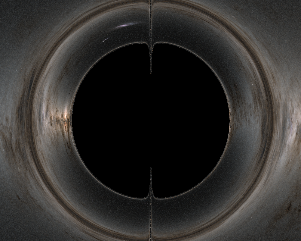
Debugging these simulations is a big pain. If you have a camera position of $(0, 5, pi/2, -pi/2)$ and use an fov of $90^o$, you’ll end up with the above picture for $r_s = 1$. The code accompanying this article can be found on the blog’s repository, with the main file here. Its only dependencies are SFML, and a tensor implementation (so checkout with submodules). I would recommend compiling with -O3 -ffast-math -NDEBUG
The first thing you might notice when putting all this together, is that it is excruciatingly slow to render a black hole, even with multiple threads. This problem is embarrassingly parallel, so next time round, we’ll be porting the whole thing to the gpu - as well as building ourselves a custom high performance GPU programming language to use
The second thing you might notice is those classic very ugly polar singularities. This can be alleviated by lowering the timestep near the poles, or by exploiting the spherical symmetry of the metric to move rays into a plane where there is no polar singularity
That’s the end of this article though, and we’ll be moving on to greener pastures. Do note, this is the most general form of integrator for general relativity, and what we’ve built can handle any spacetime. You should be able to take a fresh metric tensor, and a set of tetrads from this22 paper, and simply replace the ones we’ve coded in. I’d recommend 2.17.1, as we will be revisiting kerr in a future article and you can check your workings
As always, I’ve implemented all of this in a free tool called the Relativity Workshop, which you can use to fly around black holes and a lot more in realtime. If anyone needs a physics guy to do cool physics stuff, that’d also be pretty neat
Footnote: Indices examples
I am a pattern matcher by nature, so here’s a bunch of examples
\[\begin{aligned} &\partial_\mu \beta^\mu &&= \partial_0 \beta^0 + \partial_1 \beta^1 + \partial_2 \beta^2 + \partial_3 \beta^3 \\ \\ &A_{ij} \partial_m \beta^m &&= A_{ij}(\partial_0 \beta^0 + \partial_1 \beta^1 + \partial_2 \beta^2 + \partial_3 \beta^3)\\ \\ &\Gamma^m \partial_m \beta^i &&= \Gamma^0 \partial_0 \beta^i + \Gamma^1 \partial_1 \beta^i + \Gamma^2 \partial_2 \beta^i + \Gamma^3 \partial_3 \beta^i \\ \\ &A_{im} A^m_{\;\;j} &&= A_{i0} A^0_{\;\;j} + A_{i1} A^1_{\;\;j} + A_{i2} A^2_{\;\;j} + A_{i3} A^3_{\;\;j} = B_{ij}\\ \\ &\gamma^{mn} D_m A_{ni} - \frac{3}{2} A^m_{\;\;i} \frac{\partial_m \chi}{\chi} &&= \sum_{m=0}^3 \sum_{n=0}^3 \gamma^{mn} D_mA_{ni} - \frac{3}{2\chi} \sum_{m=0}^3 A^m_{\;\;i} \partial_m \chi \\ \\ &A^{im} (3\alpha \frac{\partial_m \chi}{\chi} + 2\partial_m \alpha) &&= \sum_{m=0}^3 A^{im} (3\alpha \frac{\partial_m \chi}{\chi} + 2\partial_m \alpha) = \frac{3 \alpha}{\chi}\sum_{m=0}^3 A^{im} \partial_m \chi + 2 \sum_{m=0}^3 \partial_m \alpha \\ \end{aligned}\]Raising and lowering examples
\[\begin{aligned} A^\mu_{\;\;\nu} &= g^{\mu k} A_{k\nu} \\ \\ A_\mu^{\;\;\nu} &= g^{\nu k} A_{\mu k} \\ \\ A^{\mu\nu} &= g^{\mu m}g^{\nu k} A_{mk} \\ \\ A_\mu^{\;\;\nu} &= g_{\mu k} A^{k\nu} \\ \\ A^\mu_{\;\;\nu} &= g_{k \nu} A^{\mu k} \\ \\ A_{\mu\nu} &= g_{\mu m}g_{\nu k} A^{mk} \\ \end{aligned}\]The rules are exactly the same for higher dimensional objects:
\[\Gamma^{\mu\nu}_{\;\;\;\sigma} = g^{\nu\gamma} \Gamma^\mu_{\;\;\gamma\sigma}\] \[\Gamma_{\mu\nu\sigma} = g_{\mu\gamma} \Gamma^{\gamma}_{\;\;\nu\sigma}\]Remember that the metric tensor is always symmetric, so we could also write this
\[\Gamma_{\mu\nu\sigma} = g_{\gamma\mu} \Gamma^{\gamma}_{\;\;\nu\sigma}\]When reading partial derivatives with raise indices, be careful: The expression $\partial_{\mu} \beta^{\nu}$ probably doesn’t mean this:
\[\partial_{\mu} \beta^{\nu} = g^{k\nu} (\partial_{\mu} \beta_k)\]But instead
\[\partial_{\mu} \beta^{\nu} = \partial_{\mu} (g^{k\nu} \beta_k)\]Here I introduce some of the slightly more obscure notation
\[\begin{aligned} \partial^\mu \beta_\nu &= g^{\mu k} \partial_k \beta_\nu \\ \\ A_{ij,}^{\;\;\;\;k} &= \partial^k A_{ij} = g^{mk} \partial_m A_{ij}\\ \end{aligned}\]One other fun thing is that derivatives are often juggled like they are variables, so keep an eye out for that
\[(\partial_k + 2) A_{ij} = \partial_k A_{ij} + 2A_{ij}\]Footnote: The metric tensor as a partial function
Earlier, we considered the metric tensor as a function taking two arguments, $g(u,v)$. One helpful way to look at covariant and contravariant indices is as partial function applications of the metric tensor:
\[u_\mu v^\mu == u^\mu v_\mu == g_{\mu\nu} u^\nu v^\mu == g^{\mu\nu} u_\nu v_\mu == g(u, v) == g(u, \cdot) \circ v\]That is to say, we can treat applying the metric tensor to $u^\mu$ to get $u_\mu$, then applying that to $v^\nu$, like currying
Further reading
A good article by a friend on geodesics in the hamiltonian formalism
A CPU raytracer, which was a primary source when I started learning, and an extremely valuable reference. Note it uses the opposite metric signature convention, so some translating has to be done
If you need any help, or you get stuck, please feel free to send me a message or email me, I’m always happy to help!
-
If someone hired me to do this full time I’d be very happy ↩
-
Black holes have no mass, in a relativistic stress-energy-tensor sense. This might be confusing, because A: Everyone talks about the mass of a black hole, and B: stuff clearly orbits a black hole. What black holes actually have is a mass equivalent parameter, which is often called $M$, and the effect that a black hole has on spacetime is equivalent to a mass-ive body with that mass. This effect is often referred to as mass, but is not the same thing as the everyday concept of mass. This level of pedantry is necessary in the future, when we will begin to struggle with what we mean by mass. In the general case, there is no single definition for the mass of a black hole, and in some cases it is undefineable ↩ ↩2
-
Basis vectors are the direction vectors of our coordinate system that we use to build our own vectors on top of. When you have a vector $(1, 2, 3)$, its generally implicit in the definition that each of these components refers to a different direction in your coordinate system, where the direction is dependent on your basis vectors. Normally your basis vectors are something like $(1,0,0)$, $(0,1,0)$, $(0,0,1)$ for x, y, and z - but in theory they could be anything - as long as they’re ‘linearly independent’. All that means is that we aren’t repeating ourselves with our basis vectors, and they truly represent different directions ↩
-
Contravariant vectors are so called because when your coordinate system changes, they scale against the axis. Eg if you have a position 0.1 in meters, and your coordinate system changes to kilometers, you have 0.1/1000 km. Covariant vectors change with the axis. Invariance is something that does not change with a change in the coordinate system, eg scalar values
A good mnemonic for remembering which is an up index, and which is a down index, is that up indices are contravariant, and down indices are covariant. But seriously, you just have to remember it ↩ ↩2
-
This example object is generally written slightly more compactly, as $ \Gamma^\mu_{\nu\sigma} $, and is known as “christoffel symbols of the second kind”. In the literature, the notation can be slightly ambiguous as to which specific index in an object is raised or lowered, and you have to deduce it from context ↩
-
These objects are often all referred to as “tensors”, a term which has lost virtually all meaning in computer science, and is struggling in physics as well. In its strict definition, a tensor is an object that transforms in a particular fashion in a coordinate change: in practice, everyone calls everything a tensor, unless its relevant for it not to be. Here, we will refer to anything which takes an index as being a tensor, unless it is relevant. The other important class of objects are scalars, which are just values ↩
-
This is generally never true of any other object, and $ A^{\mu\nu} = (A_{\mu\nu})^{-1} $ is likely a mistake ↩
-
Or any particle without rest mass. Do note that light does have mass, it just doesn’t have rest mass. It shows up in the stress-energy tensor as a result, and exerts a force of gravity ↩
-
Its also common to use the following definitions for timelike and spacelike geodesics in terms of the spacetime interval
- If $g_{\mu\nu} v^\mu v^\nu == 1$, our curve is spacelike
- If $g_{\mu\nu} v^\mu v^\nu == -1$, our curve is timelike
These different definitions correspond to particular choices for the parameterisation $ds$ for our geodesics velocity $v^\mu = \frac{dx^\mu}{ds}$: for timelike geodesics, $ds_{parameter}=-d\tau$, if $g_{\mu\nu} v^\mu v^\nu == -1$. This basically says that the geodesic becomes parameterised by proper time, and $v^\mu == \frac{dx}{d\tau}$. This is very useful, as it allows us to directly trace a geodesic based on the observers own experience of their time ↩
-
An affine parameter is so called because there are a series of parameters related by affine transforms $a * ds + b$, that are compatible with each other. If we apply something that isn’t an affine transform to our parameter, we need to modify the geodesic equation to suit
The coordinate time version of a geodesic, $\frac{dx^\mu}{dt}$ is not affinely related to $ds$, and therefore the coordinate time geodesic equation involves some extra terms.
For timelike rays, $d\tau$ is affinely related to $ds$, and therefore we can set the parameter $ds$ to $d\tau$ and use the same geodesic equation. In units of c=1, if $g_{\mu\nu} v^{\mu} v^{\nu} = -1$ (which you make true by construction), then $ds = d\tau$. If $g_{\mu\nu} v^{\mu} v^{\nu} != -1$, $ds$ and $d\tau$ are related by a scaling factor
It should be noted that as we trace forwards a path, any vectors associated with that path that are transported along it have their inner products preserved. This is a fancier way of saying that if $g_{\mu\nu} v^{\mu} v^{\nu} = -1$, it will remain true along the whole path ↩
-
Bear in mind that we’re just multiplying scalar values together here, so we can do all the sums individually. That is to say, $ \Gamma^\mu_{\alpha\beta} = \frac{1}{2} g^{\mu\sigma} (g_{\sigma\alpha,\beta} + g_{\sigma\beta,\alpha} - g_{\alpha\beta,\sigma}) $ == $ \frac{1}{2} g^{\mu\sigma} g_{\sigma\alpha,\beta} + \frac{1}{2} g^{\mu\sigma}g_{\sigma\beta,\alpha} - \frac{1}{2} g^{\mu\sigma}g_{\alpha\beta,\sigma} $. Note that we apply the derivative first, then multiply. Expressions are often constructed to avoid these kind of ambiguity, by introducing intermediate tensors ↩
-
Note: There are two sign conventions in general relativity, [+,-,-,-], and [-,+,+,+]. Wikipedia tends to use a mix - in that article, it uses the former. This tutorial series exclusively uses the latter, which is why our metric’s sign is flipped vs wikipedia
In the [+,-,-,-] convention which we do not use, the signs for spacelike, and timelike geodesics are flipped when classifying them them with the spacetime interval $ds^2$ ↩ ↩2
-
The line element can also be thought of as an expanded out form of when you apply your metric tensor to an infinitesimal displacement, $g(du, du)$. When $du = (dt, dr, d\theta, d\phi)$, we recover our line element ↩
-
Tensors and scalar functions are generally associated with a point in spacetime, which is their origin in a sense. More formally they are tangent vectors - tangent to the ‘manifold’ that is spacetime. Their origin is where you must calculate the metric tensor (and other tensors) to be able to do operations on them ↩
-
Catalogue of spacetimes 1.4.19 ↩
-
Note that, $g_{\mu\nu} v^\mu v^\nu = v_\mu v^\mu = 0$. This means that $v_0 v^0 = -\sum_{k=1}^3 v_k v^k$, and if the spatial length of $v$ is $1$, then a lightlike geodesic has $v_0 = \pm1$. A more intuitive derivation might be to use the line element for minkowski here: $-dt^2 + dx^2 + dy^2 + dz^2 = 0$. If $dx^2 + dy^2 + dz^2 == 1$, then $-dt^2 = -1$, and $dt = \pm 1$ ↩
-
See Catalogue of Spacetimes 1.4.21 for the direct example for diagonal metrics. In general, you can calculate this tetrad via gram schmidt orthonormalisation, treating the metric tensor as column vectors ↩
-
Do note that while it is true that the natural tetrad doesn’t inherently have any special meaning, it is common for the metrics to be constructed such that the natural tetrad does have special meaning, and the coordinate system often describes a particular kind of observer. In schwarzschild, this tetrad defines a stationary observer, as the metric was made to do this in these coordinates. A stationary observer actually accelerates away from the black hole to maintain its position, accelerating nearly infinitely fast just above the event horizon ↩