Numerical Relativity 101: Simulating spacetime on the GPU
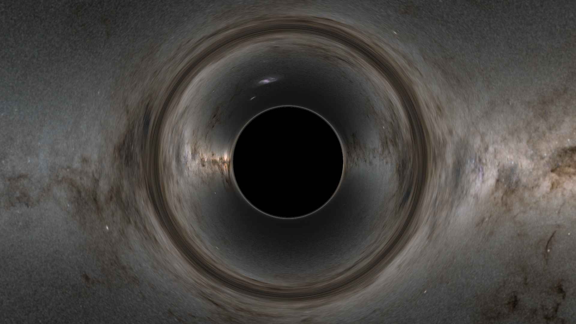
Hi there! Today we’re going to be getting into numerical relativity, which is the art of simulating the evolution of spacetime itself. While there a quite a few known solutions to the equations of general relativity at this point (eg the Schwarzschild metric), many of the most interesting regions of general relativity can only be explored by directly simulating how spacetime itself evolves dynamically. Binary black hole collisions are a perfect example of this, and are a big part of the reason why we’re building this
These kinds of simulations are traditionally run on supercomputers, but luckily you likely have a supercomputer in the form of a GPU1 in your PC. The amount of extra performance we can get over a traditional CPU based implementation is likely to be a few orders of magnitude higher if you know what you’re doing, so in this article I’m going to present to you how to get this done
If anyone’s looking for a PhD student to smash black holes together, then I’d love that. This article comes with code, which you can find over here. I would highly recommend looking at it for this article
Preamble
In this article we’ll be using the Einstein summation convention, and I’m going to assume you know how to raise and lower indices. See this article or wikipedia for more details, but the short version is:
- Objects can have raised or lowered indices, eg $v^\mu$ or $v_\mu$. These are two representations of the same object
- Repeated indices are summed, eg $v^\mu v_\mu == v^0 v_0 + v^1 v_1 + v^2 v_2 + v^3 v_3$
- Indices can be raised and lowered by the metric tensor, eg $v^\mu = g^{\mu\nu} v_\nu$, and $v_\mu = g_{\mu\nu} v^\nu$
- The inverse of the metric $g_{\mu\nu}$ - that is $g^{\mu\nu}$ - is calculated via a matrix inverse, ie $g^{\mu\nu} = (g_{\mu\nu})^{-1}$
You don’t necessarily need to understand any of this to work with the equations, just bear in mind that you can transform between the raised and lowered index forms of an object with a matrix multiplication - via the metric tensor. The (4d) metric tensor fully describes a spacetime
The ADM (Arnowitt–Deser–Misner) formalism
The Einstein field equations (EFE’s) are what defines the structure of spacetime. In general, people have come up with a variety of interesting analytic solutions to these (with a great deal of effort), including Schwarzschild, Kerr, and more
Solutions to the Einstein field equations are described in their entirety by an object called the metric tensor. For our purposes, you can think of this as a 4x4 matrix2. For a Schwarzschild black hole, that looks like this:
| $g_{\mu\nu}$ | 0 | 1 | 2 | 3 |
|---|---|---|---|---|
| 0 | $-(1-\frac{r_s}{r})$ | 0 | 0 | 0 |
| 1 | 0 | $(1-\frac{r_s}{r})^{-1}$ | 0 | 0 |
| 2 | 0 | 0 | $r^2$ | 0 |
| 3 | 0 | 0 | 0 | $r^2 sin^2(\theta)$ |
With a coordinate system $(t, r, \theta, \phi)$. Its notable that this solution describes spacetime both in the future, and in the past - relative to whenever you exist - it is defined over all time. This brings up the fundamental question that we need to solve: What happens if we only have a solution for ‘now’, and we want to instead simulate what the future would look like?
The ADM formalism is the most widespread approach for handling this. It consists of slicing a 4d spacetime explicitly into a series (foliation) of 3d spacelike slices (hypersurfaces), and separates out a timelike dimension which traverses these. It is often referred to as a “3+1” formalism as a result. You can imagine this like a series of stacked sheets that you can traverse
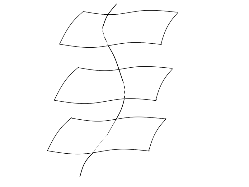
Each sheet represents one slice that we can call ‘now’, although that’s stretching the terminology a bit. The slices themselves can be pretty arbitrary - the important thing is that you can define how one slice changes into the next, and so work out how spacetime evolves into the future if we’re able to fully determine the structure of any individual slice
Realistically, I’m not very good at art, so if you want a good intuitive picture to refer back to, I’d recommend page 12
Details
From now on, all latin indices \(_{ijk}\) have the value 1-3, and generally denote quantities on our 3d slice, whereas greek indices \(_{\mu\nu\kappa}\) take on the value 0-3 and denote quantities in our 4d spacetime
The general line element in ADM is this:
\[ds^2 = -\alpha^2 dt^2 + \gamma_{ij} (dx^i + \beta^i dt)(dx^j + \beta^jdt)\]Or, as a 4x4 matrix again:
| $g_{\mu\nu}$ | $0$ | $i$ |
|---|---|---|
| $0$ | $-\alpha^2 + \beta_m \beta^m$ | $\beta_i$ |
| $j$ | $\beta_j$ | $\gamma_{ij}$ |
This is the most general form of the ADM metric, and dictates how we chop up our general3 4d spacetime into our 3+1d components. The variables introduced here are as follows:
| Variable | Definition |
|---|---|
| $\gamma_{ij}$ | The metric tensor on our 3d slice, sometimes called the ‘induced’ metric |
| $K_{ij}$ | The extrinsic curvature. It represents the embedding of our 3d slice in the larger 4d spacetime. It can be thought of as a momentum term for $\gamma_{ij}$ |
| $\alpha$4 | The lapse, a gauge variable, which is related to the separation between slices5 |
| $\beta^i$4 | The shift, another gauge variable, related to how a point moves from one slice to the next5 |
$\gamma_{ij}$ can be used to raise and lower indices on a 3d slice as per usual6. Eg, given a tensor $Q_i$
\[\begin{align} Q^i &= \gamma^{ij} Q_j \\ Q_i &= \gamma_{ij} Q^j \end{align}\]If our 4-metric is $g_{\mu\nu}$, then the 3-metric is $\gamma_{ij} = g_{ij}$, ie the spatial parts. While $\gamma^{ij} = (\gamma_{ij})^{-1}$ (the 3x3 matrix inverse), $\gamma^{ij} \neq g^{ij}$
Equations of motion
The ADM formalism has equations of motion associated with it - defining the evolution of the metric and extrinsic curvature in time. These can be derived by defining a Lagrangian, and using standard techniques on it. Once that’s all done, the ADM equations of motion can be brought into the following form7:
\[\begin{align} \partial_t \gamma_{ij} &= \mathcal{L}_\beta \gamma_{ij} - 2 \alpha K_{ij}\\ \partial_t K_{ij} &= \mathcal{L}_\beta K_{ij} - D_i D_j \alpha + \alpha (R_{ij} - 2 K_{il} K^l_j + K K_{ij}) \end{align}\]Where $\mathcal{L}_\beta$ is a lie derivative, and $D_i$ is the covariant derivative associated with \(\gamma_{ij}\). We must also provide adequate gauge conditions (evolution equations for the gauge variables), and then in theory you have a fully working formalism for evolving a slice of spacetime into the future
Unfortunately, there’s a small problem
The ADM equations of motion are bad

Part of the reason why we’re not going into this more is that - unfortunately - these equations of motion are unusable to us. They are very numerically unstable, to the point where for our purposes8 there’s no point trying to solve them. Understanding this issue, and solving it was an outstanding problem for decades, and there is an absolutely enormous amount written in the literature on this topic. A lot of this article series is going to be dealing with the very poor character of the equations
Luckily, because its not the early 2000s - and because the astrophysics community rocks and makes all this information public - we get to skip to the part where we have a workable set of equations
Enter: The BSSN formalism
The BSSN formalism is the most widely used formalism and what we’ll actually be implementing - it is directly derived from the ADM formalism, and most practical formalisms are substantially similar to the BSSN formalism. It was the first very successful formalism to enter the picture - though it was unclear precisely why it worked so well for a long time9
There are 4 main ingredients to get the BSSN equations from the ADM equations:
- The metric $\gamma_{ij}$ is split into a metric with unit determinant \(\tilde{\gamma}_{ij}\), and a conformal (scalar) factor. This is called a conformal decomposition
- The extrinsic curvature $K_{ij}$ is split up into its trace: $K$, and the conformal trace free part of the extrinsic curvature, \(\tilde{A}_{ij}\)
- A new redundant variable \(\tilde{\Gamma}^i = \tilde{\gamma}^{mn} \tilde{\Gamma}^{i}_{mn}\)10 is introduced and evolved dynamically, which eliminates a major source of numerical instabilities11
- The constraints are substituted in to eliminate numerically unstable quantities12
With all this applied, you end up with the BSSN formalism. We’ll go through the relevant elements of this now
Conformal decomposition
The two non-gauge ADM variables are: $\gamma_{ij}$ the metric tensor, and $K_{ij}$, the extrinsic curvature, and these are what we’ll split up - via what’s called the $W^2$ conformal factor. This is used to define the conformal metric tensor13 as follows:
\[\tilde{\gamma}_{ij} = W^2 \gamma_{ij}\]The inverse of the metric is also straightforward:
\[\begin{align} W^2 \tilde{\gamma}^{ij} &= \gamma^{ij}\\ \tilde{\gamma}^{ij} &= (\tilde{\gamma}_{ij})^{-1} \end{align}\]\(K_{ij}\) is split into its trace $K = \gamma^{mn} K_{mn}$, and the conformal trace-free part called \(\tilde{A}_{ij}\)
\[\tilde{A}_{ij} = W^2 (K_{ij} - \frac{1}{3} \gamma_{ij} K) = W^2 (K_{ij})^{TF}\]If you’re wondering $W$ is squared rather than a non squared conformal variable (which is used in the literature), please see the discussion on conformal factors at the end of this article for a discussion on the alternatives
Variables
The full set of BSSN variables after conformally decomposing $\gamma_{ij}$ and $K_{ij}$ is as follows:
\[\begin{align} &\tilde{\gamma}_{ij} &&= W^2 \gamma_{ij}\\ &\tilde{A}_{ij} &&= W^2 (K_{ij} - \frac{1}{3} \gamma_{ij} K)\\ &K &&= \gamma^{mn} K_{mn}\\ &W &&= det(\gamma)^{-1/6}\\ &\tilde{\Gamma}^i &&= \tilde{\gamma}^{mn} \tilde{\Gamma}^i_{mn}\\ &\alpha_{bssn} &&= \alpha_{adm}\\ &\beta^i_{bssn} &&= \beta^i_{adm}\\ \end{align}\]Phew. Conformal variables have a tilde over them, and have their indices raised and lowered with the conformal metric tensor. In this definition, the determinant of the conformal metric is \(\tilde{\gamma} = 1\), and \(\tilde{A}_{ij}\) is trace-free. $K$ is the trace of $K_{ij}$. $K_{ij}$, $\gamma_{ij}$, \(\tilde{A}_{ij}\), and \(\tilde{\gamma}_{ij}\) are all symmetric
There are also a number of constraints that must be satisfied for the BSSN formalism to be well posed. The momentum and hamiltonian constraints come from this being derived from a Lagrangian approach, and the others are specific to the BSSN formalism
Constraints
Momentum
\[\mathcal{M}_i = \tilde{\gamma}^{mn} \tilde{D}_m \tilde{A}_{ni} - \frac{2}{3} \partial_i K - \frac{3}{2} \tilde{A}^m_{\;\;i} \frac{\partial_m \chi}{\chi} = 0\]Where \(\tilde{D}_i\) is the covariant derivative associated with \(\tilde{\gamma}_{ij}\), calculated in the usual fashion. \(\chi = W^2\)
Hamiltonian
\[\mathcal{H} = \mathcal{R} + \frac{2}{3} K^2 - \tilde{A}^{mn} \tilde{A}_{mn} = 0\]Where $\mathcal{R}$ is the trace of \(\mathcal{R}_{ij}\) with respect to \(\gamma_{ij}\) (ie \(\mathcal{R}_{ij} \gamma^{ij}\)), and will be introduced in full later
Algebraic
\[\begin{align} \mathcal{S} &= \tilde{\gamma} - 1 &= 0\\ \mathcal{A} &= \tilde{\gamma}^{mn} \tilde{A}_{mn} &= 0 \end{align}\]Where \(\tilde{\gamma}\) is the determinant of the metric. These constraints mean that the determinant of the metric should be $1$, and the trace of \(\tilde{A}_{ij}\) should be 0
Christoffel symbol
\[\mathcal{G}^i = \tilde{\Gamma}^i - \tilde{\gamma}^{mn} \tilde{\Gamma}^i_{mn} = 0\]Constraint summary
Ensuring that the constraints don’t blow up numerically is key to making the BSSN formalism work, so we’ll be getting back to all of these. The only one you can largely ignore is the hamiltonian constraint - and for this article, the christoffel symbol constraint is unused
Equations of motion
I’m going to present to you the14 canonical form of the BSSN equations, and then discuss how you might want to rearrange them a bit in practice afterwards
\[\begin{align} \partial_t W &= \beta^m \partial_m W + \frac{1}{3} W (\alpha K - \partial_m \beta^m) \\ \partial_t \tilde{\gamma}_{ij} &= \beta^m \partial_m \tilde{\gamma}_{ij}+ 2 \tilde{\gamma}_{m(i} \partial_{j)} \beta^m - \frac{2}{3} \tilde{\gamma}_{ij} \partial_m \beta^m - 2 \alpha \tilde{A}_{ij} \\ \partial_t K &= \beta^m \partial_m K - W^2 \tilde{\gamma}^{mn} D_m D_n \alpha + \alpha \tilde{A}^{mn} \tilde{A}_{mn} + \frac{1}{3} \alpha K^2\\ \partial_t \tilde{A}_{ij} &= \beta^m \partial_m \tilde{A}_{ij}+ 2 \tilde{A}_{m(i} \partial_{j)} \beta^m - \frac{2}{3} \tilde{A}_{ij} \partial_m \beta^m + \alpha K \tilde{A}_{ij} \\&- 2 \alpha \tilde{A}_{im} \tilde{A}^m_{\;\;j} + W^2 (\alpha \mathcal{R}_{ij} - D_i D_j \alpha)^{TF} \\ \partial_t \tilde{\Gamma}^i &= \beta^m \partial_m \tilde{\Gamma}^i + \frac{2}{3} \tilde{\Gamma}^i \partial_m \beta^m - \tilde{\Gamma}^m \partial_m \beta^i + \tilde{\gamma}^{mn} \partial_m \partial_n \beta^i + \frac{1}{3} \tilde{\gamma}^{im} \partial_m \partial_n \beta^n \\ &-\tilde{A}^{im}(6\alpha \frac{\partial_m W}{W} + 2 \partial_m \alpha) + 2 \alpha \tilde{\Gamma}^i_{mn}\tilde{A}^{mn} - \frac{4}{3} \alpha \tilde{\gamma}^{im} \partial_m K \end{align}\]With the secondary expressions:
\[\begin{align} \mathcal{R}_{ij} &= \tilde{\mathcal{R}}_{ij} + \mathcal{R}^W_{ij}\\ \mathcal{R}^W_{ij} &= \frac{1}{W^2} (W (\tilde{D}_i \tilde{D}_j W + \tilde{\gamma}_{ij} \tilde{D}^m \tilde{D}_m W) - 2 \tilde{\gamma}_{ij} \partial^m W \partial_m W)\\ \tilde{\mathcal{R}}_{ij} &= -\frac{1}{2} \tilde{\gamma}^{mn} \partial_m \partial_n \tilde{\gamma}_{ij} + \tilde{\gamma}_{m(i} \partial _{j)} \tilde{\Gamma}^m + \tilde{\Gamma}^m \tilde{\Gamma}_{(ij)m}+ \tilde{\gamma}^{mn} (2 \tilde{\Gamma}^k_{m(i} \tilde{\Gamma}_{j)kn} + \tilde{\Gamma}^k_{im} \tilde{\Gamma}_{kjn})\\ D_iD_j\alpha &= \tilde{D}_i \tilde{D}_j \alpha + \frac{2}{W} \partial_{(i} W \partial_{j)} \alpha\ - \frac{1}{W} \tilde{\gamma}_{ij} \tilde{\gamma}^{mn} \partial_m W \partial_n \alpha \end{align}\]Additionally:
-
\(^{TF}\) means to take the trace free part of a tensor, calculated as \(Q_{ij}^{TF} = Q_{ij} - \frac{1}{3} \tilde{\gamma}_{ij} \tilde{\gamma}^{mn} Q_{mn} = Q_{ij} - \frac{1}{3} \tilde{\gamma}_{ij} Q\).15
-
The symmetrising operator crops up here unintuitively. This is defined as $A_{(ij)}$ = $0.5 (A_{ij} + A_{ji})$. A more complex example is \(2\tilde{\Gamma}^k_{m(i} \tilde{\Gamma}_{j)kn} = 0.5 * 2 (\tilde{\Gamma}^k_{mi} \tilde{\Gamma}_{jkn} + \tilde{\Gamma}^k_{mj} \tilde{\Gamma}_{ikn})\)
-
Raised indices on covariant derivatives mean this: \(\tilde{D}^i = \tilde{\gamma}^{ij} \tilde{D}_j\). The same is true for partial derivatives, ie \(\partial^i = \tilde{\gamma}^{ij} \partial_j\)
This is fairly dense as things go, and if you’re going to implement this there isn’t really a solid strategy other than to just dig in and make a bunch of mistakes translating it into code. This is a big part of the reason why this article comes with a complete implementation
Gauge conditions
The ADM/BSSN formalism does not uniquely specify the evolution equations for the lapse and shift, and there is a freedom of choice here. Despite in theory being fairly arbitrary, in practice you have to very carefully pick your gauge conditions for the kind of problem you’re trying to solve. For today, we’re going to be picking what’s called the harmonic gauge (aka harmonic slicing), with 0 shift:
\[\begin{align} \partial_t \alpha &= - \alpha^2 K + \beta^m \partial_m \alpha\\ \beta^i &= 0 \end{align}\]The reason to use this specific form is just to replicate paper results for today’s test case - and I’m glossing over gauge conditions a bit here because they’ll become much more relevant when we collide black holes together. See the end of the article for more discussion around gauge conditions
The BSSN equations of motion are bad

So, as written, the BSSN equations of motion are - drumroll - very numerically unstable, and attempting to directly implement the PDEs listed above will result in nothing working. I’ll attempt to briefly summarise several decades of the conventional wisdom from stability analysis here16 on how to fix this:
- If the second algebraic constraint $\mathcal{A}$ is violated, ie the trace of the trace-free extrinsic curvature != 0, the violation blows up and your simulation will virtually immediately fail
- Correcting momentum constraint $\mathcal{M}_i$ violations is very important
- The christoffel symbol constraint $\mathcal{G}^i$ is quite important to damp
Additionally:
- Hamiltonian constraint violations are essentially unimportant for stability purposes, and damping this seems to be largely irrelevant for physical accuracy
- The first algebraic constraint $\mathcal{S}$ is relatively unimportant to enforce, but its easy to do - so we may as well
Expressions involving undifferentiated $\tilde{\Gamma}^i$’s are frequently replaced in the literature with the analytic equivalent \(\tilde{\gamma}^{mn} \tilde{\Gamma}^i_{mn}\). This is one technique to enforce the $\mathcal{G}^i$ constraint, though we’re going to avoid this approach because it only really works well in specific circumstances (that we’ll get into in the future)
Fixing the BSSN equations
Before we can get off the ground, we’re going to have to at minimum implement the following three things
- Algebraic constraint enforcement
- Momentum constraint damping
- Numerical dissipation
The algebraic constraints
The most common technique for dealing with the algebraic constraints is to enforce the relation $\tilde{\gamma} = 1$ and $\tilde{\gamma}^{mn} \tilde{A}_{mn} = 0$ directly. This is easily done by applying the following expressions:
\[\begin{align} \tilde{\gamma}_{ij} &= \frac{\tilde{\gamma}_{ij}}{\tilde{\gamma}^\frac{1}{3}} \\ \tilde{A}_{ij} &= \tilde{A}_{ij}^{TF} \end{align}\]There’s some discussion about alternatives at the end of this article
The Momentum constraint
The most common way of damping momentum constraint errors is as follows:
\[\partial_t \tilde{A}_{ij} = \partial_t \tilde{A}_{ij} + k_m \alpha \tilde{D}_{(i} \mathcal{M}_{j)}\]Where $k_m$ > 0. Do be aware that this is a scale dependent parameter, so if you double your resolution you’ll need to halve it
The Christoffel symbol constraint
The most straightforward way to apply this is by applying the $\mathcal{G}^i$ constraint as follows:
\[\partial_t \tilde{\Gamma}^i = \partial_t \tilde{\Gamma}^i - \sigma \mathcal{G}^i \partial_m \beta^m\]Where $\sigma$ > 0. This modification is not used in this article because $\beta^i = 0$
Other constraints
Damping the hamiltonian constraint is unnecessary here, but this paper contains some ideas that work
Dissipating Numerical Noise
Even with all the constraint damping, the equations can still be numerically unstable - the last tool in the toolbox is called Kreiss-Oliger dissipation. This essentially is a blur on your data - it extracts a certain order of frequencies from your simulation grid, and damps them. The Einstein Toolkit site gives this definition17:
\[\partial_t U = \partial_t U + (-1)^{(p+3)/2} \epsilon \frac{h^p}{2^{p+1}} (\frac{\partial^{p+1}}{\partial x^{p+1}} + \frac{\partial^{p+1}}{\partial y^{p+1}} + \frac{\partial^{p+1}}{\partial z^{p+1}})U\]$\epsilon$ is a damping factor (eg $0.25$), and $h$ is the grid spacing. $p$ is the order of the dissipation, although there appears to be some confusion about what it means18. 6th order derivatives are common to use, here I’m going to set $p=5$
\[\partial_t U = \partial_t U + \epsilon \frac{h^5}{64} (\frac{\partial^6}{\partial x^6} + \frac{\partial^6}{\partial y^6} + \frac{\partial^6}{\partial z^6})U\]There are two major ways of implementing this:
- Modifying the evolution equations as written above
- As a pure numerical filter, ie as a frequency removal pass over your data
I pick #2, as it can be implemented more efficiently, but really both work nearly identically
Note, 6th derivatives imply a division by $h^6$ - which is then immediately multiplied by $h^5$, and you may not want to do this numerically
Simulating the equations
To actually simulate the equations, we’re going to need a few more things
- An integrator to integrate the equations of motion
- Initial conditions
- Boundary conditions
Picking an integrator
The BSSN equations are a classically stiff (unstable) set of equations, which means that integrators can have a hard time providing accurate results. Its traditional to use something similar to RK4 to integrate the equations of motion
If you’re familiar with solving stiff PDEs, it might seem a bit odd to use RK4 - RK4 is an explicit integrator - and as such has fairly poor stability properties when solving stiff equations. Instead, we’re going to use an L-stable implicit integrator which has excellent convergence properties - backwards euler
Backwards euler also has a very GPU-friendly form, making it amenable to a high performance implementation, while using a minimal amount of memory - this means that the performance/step size is very favourable
Solving implicit equations efficiently
Backwards euler has the form:
\[y_{n+1} = y_n + dt f(t_{n+1}, y_{n+1})\]Where $dt$ is a timestep, and $y_n$ is our current set of variables. This is a first order integrator, and it is implicit - we have $y_{n+1}$ on both sides of the equation
Fixed point iteration
The issue with an implicit integrator is: How do we actually solve this equation? The straightforward answer is to use fixed point iteration. In essence, you feed your output to your input repeatedly. Ie, if $f(x)$ gives you your next guess, you iterate the sequence $f(x)$, $f(f(x))$, $f(f(f(x)))$, until you reach your desired accuracy
For our purposes, we’ll iterate the sequence:
\[y_{k+1, n+1} = y_n + dt f(y_{k,n+1})\]Over our iteration variable $k$. To initialise the fixed point iteration, $y_{0, n+1} = y_{n}$. This makes the first step forwards euler
This form of fixed point iteration maps very well to being implemented on a GPU, is numerically stable, and in general is extremely fast and robust. There are tricks19 to speed up fixed point iteration as well
Initial conditions
We need to define on an initial slice what our variables are. For this article, to check everything’s working we’re going to implement a gauge wave test case, which you can find here (28-29), or here (A.10 + A.6, this is what we’re actually implementing). The metric for this is as follows20 -
\[ds^2 = (1 - H) (-dt^2 + dx^2) + dy^2 + dz^2\]where
\[H = A \sin(\frac{2 \pi (x - t)}{d})\]$d$ is the wavelength of our wave, which is set to 1 (our simulation width), and $A$ is the amplitude of the wave which is set to $0.1$. On our initial slice, $t=0$. This defines a 4-metric $g_{\mu\nu}$. While these papers do provide analytic expressions for our initial ADM variables - where’s the joy in that?
Generic initial conditions
Given a metric $g_{\mu\nu}$, we want to calculate the ADM variables $\gamma_{ij}$, $K_{ij}$, $\alpha$, and $\beta^i$. From there, we already know how to take a conformal decomposition for the BSSN formalism. The relation between the ADM variables, and a regular 4d metric tensor can be deduced from the line element, but I’m going to stick it in a table for convenience:
| $g_{\mu\nu}$ | $0$ | $i$ |
|---|---|---|
| $0$ | $-\alpha^2 + \beta_m \beta^m$ | $\beta_i$ |
| $j$ | $\beta_j$ | $\gamma_{ij}$ |
| $g^{\mu\nu}$ | $0$ | $i$ |
|---|---|---|
| $0$ | $-\alpha^2$ | $\alpha^{-2} \beta^i$ |
| $j$ | $\alpha^{-2} \beta^j$ | $\gamma^{ij} - \alpha^{-2} \beta^i \beta^j$ |
With the addition of a definition for $K_{ij}$21, you end up with the following relations for our ADM variables by solving from the first table (eg, $g_{00} = -\alpha^2 + \beta_m \beta^m$):
\[\begin{align} \gamma_{ij} &= g_{ij}\\ \beta_i &= g_{0i} \\ K_{ij} &= \frac{1}{2 \alpha} (D_i \beta_j + D_j \beta_i - \frac{\partial g_{ij}}{\partial_t})\\ \alpha &= \sqrt{-g_{00} + \beta^m \beta_m} \end{align}\]Note that we find $\beta_i$ not $\beta^i$, which you can find by raising with $\gamma^{ij}$. To initialise the christoffel symbol $\tilde{\Gamma}^i$, simply calculate it analytically once you have $\tilde{\gamma}_{ij}$
Boundary conditions / Differentiation
Here, we’re going to use fourth order22 finite differentiation on a grid. If you remember, to approximate a derivative, mathematically you can do:
\[\frac{\partial f} {\partial x} = \frac{f(x+1) - f(x)}{h}\]The factor of $h$ is omitted, because we’re indexing grid cells. Numerically this is not ideal, and instead we’ll use symmetric fourth order differentiation, with coefficients which you can look up here:
\[\frac{\partial f} {\partial x} = \frac{\frac{1}{12} f(x - 2) - \frac{2}{3} f(x - 1) + \frac{2}{3} f(x + 1) - \frac{1}{12} f(x + 2)}{h}\]To take a second derivative, calculate the first derivative, then repeat the differentiation on it. 4th order differentiation tends to produce a decent tradeoff of accuracy vs performance. In this simulation, because the data is discretised onto a grid, this brings up the question of how to take derivatives at the edge of the grid (as taking derivatives involves adjacent grid cells) - solving this question defines the boundary conditions
In this test - a gauge wave - the boundary conditions are periodic, which are the simplest kind luckily. To implement this, when implementing derivatives, you wrap your coordinates to the other edge of the domain. Some performance considerations are discussed at the end of this article
Implementation
At this point, all the theory is done, so its time to get to implementing stuff. The actual code for implementing all of this can be found over here. Pasting it all in here wouldn’t really serve much purpose (because you can just go and browse the source), so this segment is going to show:
- An example of how to implement these equations
- How to differentiate things
- What equations we’re actually implementing, rather than the canonical ones
Example
The harmonic gauge condition is this:
\[\partial_t \alpha = - \alpha^2 K + \beta^m \partial_m \alpha\]Which translates directly to this:
valuef get_dtgA(bssn_args& args, bssn_derivatives& derivs, valuef scale)
{
    valuef bmdma = 0;

    for(int i=0; i < 3; i++)
    {
        bmdma += args.gB[i] * diff1(args.gA, i, scale);
    }

    return -args.gA * args.gA * args.K + bmdma;
}
In general, the equations are all just a very long sum of products. A slightly more complicated example is:
\[\partial_t W = \beta^m \partial_m W + \frac{1}{3} W (\alpha K - \partial_m \beta^m)\]valuef get_dtW(bssn_args& args, bssn_derivatives& derivs, const valuef& scale)
{
valuef dibi = 0;
for(int i=0; i < 3; i++)
{
dibi += diff1(args.gB[i], i, scale);
}
valuef dibiw = 0;
for(int i=0; i < 3; i++)
{
dibiw += args.gB[i] * diff1(args.W, i, scale);
}
return (1/3.f) * args.W * (args.gA * args.K - dibi) + dibiw;
}
Where should you diverge from the canonical equations?
Momentum constraint
The specific form of the momentum constraint I listed earlier - while a common form - involves calculating covariant derivatives which is unnecessary. A slightly better form is this:23
\[\mathcal{M_i} = \partial_j \tilde{A}_i^j - \frac{1}{2} \tilde{\gamma}^{jk} \tilde{A}_{jk,i} + 6 \partial_j \phi \tilde{A}_i^j - \frac{2}{3} \partial_i K\]Where
\[\partial_i \phi = -\frac{\partial_i W}{2 W}\]Evolution equations
-
The quantity $D_i D_j \alpha$ is never used without being multiplied by $W^2$, which means we can eliminate the divisions by $W$
-
The quantity $\mathcal{R}^W_{ij}$ is also multiplied by $W^2$, allowing us to remove the division
#2 is unique to the $W^2$ formalism, and is a very nice feature of it. In this version of BSSN, there is only one division by $W$, in the $\tilde{\Gamma}^i$ evolution equation, and you must guard against divisions by zero by clamping $W$ to a small value (eg $10^{-4}$)24
Evolving $\tilde{A}_{ij}$
\[\begin{align} \partial_t \tilde{A}_{ij} &= \beta^m \partial_m \tilde{A}_{ij}+ 2 \tilde{A}_{m(i} \partial_{j)} \beta^m - \frac{2}{3} \tilde{A}_{ij} \partial_m \beta^m + \alpha K \tilde{A}_{ij} \\&- 2 \alpha \tilde{A}_{im} \tilde{A}^m_{\;\;j} + (\alpha W^2 \mathcal{R}_{ij} - W^2 D_i D_j \alpha)^{TF} \\&+ k_m \alpha \tilde{D}_{(i} \mathcal{M}_{j)} \end{align}\]Is what we’re actually implementing. There are several modifications made here:
- The $W^2$ term is moved inside the trace free operation
- $W^2 D_i D_j \alpha$ is calculated, instead of $D_i D_j \alpha$
- \(W^2 \mathcal{R}_{ij}\) is calculated instead of \(\mathcal{R}_{ij}\)
- Momentum constraint damping has been added
\(W^2 D_iD_j\alpha\)
\[W^2 D_iD_j\alpha = W^2 \tilde{D}_i \tilde{D}_j \alpha + 2W \partial_{(i} W \partial_{j)} \alpha\ - W \tilde{\gamma}_{ij} \tilde{\gamma}^{mn} \partial_m W \partial_n \alpha\]\(W^2 \mathcal{R}_{ij}\)
\[\begin{align} W^2 \mathcal{R}^W_{ij} &= W (\tilde{D}_i \tilde{D}_j W + \tilde{\gamma}_{ij} \tilde{D}^m \tilde{D}_m W) - 2 \tilde{\gamma}_{ij} \partial^m W \partial_m W \\ W^2 \mathcal{R}_{ij} &= W^2 \tilde{\mathcal{R}}_{ij} + W^2 \mathcal{R}^W_{ij} \end{align}\]Algebraic constraint enforcement
This is straightforward:
valuef det_cY = pow(cY.det(), 1.f/3.f);

metric<valuef, 3, 3> fixed_cY = cY / det_cY;
tensor<valuef, 3, 3> fixed_cA = trace_free(cA, fixed_cY, fixed_cY.invert());
Initial conditions
The code for the initial conditions can be found here:
This is the actual metric tensor we’re using, with a generic argument so that its easy to plug in dual numbers (which is how I differentiate things here):
auto wave_function = []<typename T>(const tensor<T, 4>& position)
{
    float A = 0.1f;
    float d = 1;

    auto H = A * sin(2 * std::numbers::pi_v<float> * (position.y() - position.x()) / d);

    metric<T, 4, 4> m;
    m[0, 0] = -1 * (1 - H);
    m[1, 1] = (1 - H);
    m[2, 2] = 1;
    m[3, 3] = 1;

    return m;
};
Building the ADM variables
This isn’t too complicated to implement, though you will need the ability to differentiate your metric tensor (either numerically, or analytically)
struct adm_variables
{
    metric<valuef, 3, 3> Yij;
    tensor<valuef, 3, 3> Kij;
    valuef gA;
    tensor<valuef, 3> gB;
};

template<typename T>
adm_variables make_adm_variables(T&& func, v4f position)
{
    using namespace single_source;

    adm_variables adm;

    metric<valuef, 4, 4> Guv = func(position);

    tensor<valuef, 4, 4, 4> dGuv;

    for(int k=0; k < 4; k++)
    {
        auto ldguv = diff_analytic(func, position, k);

        for(int i=0; i < 4; i++)
        {
            for(int j=0; j < 4; j++)
            {
                dGuv[k, i, j] = ldguv[i, j];
            }
        }
    }

    metric<valuef, 3, 3> Yij;

    for(int i=0; i < 3; i++)
    {
        for(int j=0; j < 3; j++)
        {
            Yij[i, j] = Guv[i+1, j+1];
        }
    }

    tensor<valuef, 3, 3, 3> Yij_derivatives;

    for(int k=0; k < 3; k++)
    {
        for(int i=0; i < 3; i++)
        {
            for(int j=0; j < 3; j++)
            {
                Yij_derivatives[k, i, j] = dGuv[k+1, i+1, j+1];
            }
        }
    }

    tensor<valuef, 3, 3, 3> Yij_christoffel = christoffel_symbols_2(Yij.invert(), Yij_derivatives);

    pin(Yij_christoffel);

    tensor<valuef, 3> gB_lower;
    tensor<valuef, 3, 3> dgB_lower;

    for(int i=0; i < 3; i++)
    {
        gB_lower[i] = Guv[0, i+1];

        for(int k=0; k < 3; k++)
        {
            dgB_lower[k, i] = dGuv[k+1, 0, i+1];
        }
    }

    tensor<valuef, 3> gB = raise_index(gB_lower, Yij.invert(), 0);

    pin(gB);

    valuef gB_sum = sum_multiply(gB, gB_lower);

    valuef gA = sqrt(-Guv[0, 0] + gB_sum);

    ///https://clas.ucdenver.edu/math-clinic/sites/default/files/attached-files/master_project_mach_.pdf 4-19a
    tensor<valuef, 3, 3> gBjDi = covariant_derivative_low_vec(gB_lower, dgB_lower, Yij_christoffel);

    pin(gBjDi);

    tensor<valuef, 3, 3> Kij;

    for(int i=0; i < 3; i++)
    {
        for(int j=0; j < 3; j++)
        {
            Kij[i, j] = (1/(2 * gA)) * (gBjDi[j, i] + gBjDi[i, j] - dGuv[0, i+1, j+1]);
        }
    }

    adm.Yij = Yij;
    adm.Kij = Kij;
    adm.gA = gA;
    adm.gB = gB;

    return adm;
}
Building the BSSN variables
Once you have the ADM variables, its straightforward to perform the conformal decomposition, and calculate the BSSN variables
    adm_variables adm = make_adm_variables(wave_function, {0, wpos.x(), wpos.y(), wpos.z()});

    valuef W = pow(adm.Yij.det(), -1/6.f);
    metric<valuef, 3, 3> cY = W*W * adm.Yij;
    valuef K = trace(adm.Kij, adm.Yij.invert());

    tensor<valuef, 3, 3> cA = W*W * (adm.Kij - (1.f/3.f) * adm.Yij.to_tensor() * K);
Calculating the christoffel symbol is left as a separate post processing step (because directly differentiating \(\tilde{\gamma}_{ij}\) is a bit troublesome in the scheme I’ve got set up, but there’s no theoretical reason for it)
Derivatives + Boundary conditions
The boundary conditions are implemented whenever we need to take a derivative of something, and so the two topics are tied together
Below is how I generate the adjacent grid cells, so we can apply finite difference coefficients to them. The scheme I’ve set up for doing this is worth going over
///takes a memory access like v[pos, dim], and generates the sequence
///v[pos - {2, 0, 0}, dim], v[pos - {1, 0, 0}, dim], v[pos, dim], v[pos + {1, 0, 0}, dim], v[pos + {2, 0, 0}, dim]
///though in the grid direction pointed to by "direction"
template<std::size_t elements = 5, typename T>
auto get_differentiation_variables(const T& in, int direction)
{
    std::array<T, elements> vars;

    ///for each element, ie x-2, x-1, x, x+1, x+2
    for(int i=0; i < elements; i++)
    {
        ///assign to the original element, ie x
        vars[i] = in;

        ///for every argument, and ourselves
        vars[i].recurse([&i, direction](value_base& v)
        {
            ///check if we're indexing a memory location
            if(v.type == value_impl::op::BRACKET)
            {
                //if so, substitute our memory access with an offset one, for whichever coefficent we want
                auto get_substitution = [&i, direction](const value_base& v)
                {
                    assert(v.args.size() == 8);

                    ///the encoding format for the bracket operator is
                    ///buffer name, argument number, pos[0], pos[1], pos[2], dim[0], dim[1], dim[2]
                    auto buf = v.args[0];

                    ///pull out the position
                    std::array<value_base, 3> pos = {v.args[2], v.args[3], v.args[4]};
                    ///pull out the array dimensions
                    std::array<value_base, 3> dim = {v.args[5], v.args[6], v.args[7]};

                    ///generates the sequence -2, -1, 0, 1, 2 for elements=5, ie grid index offsets
                    int offset = i - (elements - 1)/2;

                    ///update our position
                    pos[direction] = pos[direction] + valuei(offset);

                    ///implement the periodic boundary
                    if(offset > 0)
                        pos[direction] = ternary(pos[direction] >= dim[direction], pos[direction] - dim[direction], pos[direction]);

                    if(offset < 0)
                        pos[direction] = ternary(pos[direction] < valuei(0), pos[direction] + dim[direction], pos[direction]);

                    ///create a new memory indexing operation with our new position
                    value_base op;
                    op.type = value_impl::op::BRACKET;
                    op.args = {buf, value<int>(3), pos[0], pos[1], pos[2], dim[0], dim[1], dim[2]};
                    op.concrete = get_interior_type(T());

                    return op;
                };

                v = get_substitution(v);
            }
        });
    }

    return vars;
}
Then this is a traditional 4th order finite difference scheme:
valuef diff1(const valuef& in, int direction, const valuef& scale)
{
    ///4th order derivatives
    std::array<valuef, 5> vars = get_differentiation_variables(in, direction);

    ///implemented like this, so that we have floating point symmetry in a symmetric grid
    valuef p1 = -vars[4] + vars[0];
    valuef p2 = 8.f * (vars[3] - vars[1]);

    return (p1 + p2) / (12.f * scale);
}

///this uses the commutativity of partial derivatives to lopsidedly prefer differentiating dy in the x direction
///as this is better on the memory layout
valuef diff2(const valuef& in, int idx, int idy, const valuef& dx, const valuef& dy, const valuef& scale)
{
    using namespace single_source;

    if(idx < idy)
    {
        ///we must use dy, therefore swap all instances of diff1 in idy -> dy
        alias(diff1(in, idy, scale), dy);

        return diff1(dy, idx, scale);
    }
    else
    {
        ///we must use dx, therefore swap all instances of diff1 in idx -> dx
        alias(diff1(in, idx, scale), dx);

        return diff1(dx, idy, scale);
    }
}
The way that this is implemented code-wise is slightly unusual. All variables in this simulation are bound to a particular grid location - eg K = K_buffer[pos, dim]. This is to minimise the complexity of the equations
Because of this, instead of having a buffer and a position to differentiate at, I have a variable which is derived from a buffer, and an expression tree containing a bracket operator - with the indexing position and dimension as arguments. The huge upside of this is being able to differentiate compound expressions, like this:
diff1(cY * cA, 0, scale);
You can look through all the internal buffer accesses, and perform the substitution on all of them to correctly differentiate this. To illustrate this in one dimension, you end up with this:
cY[x - 2] * cA[x - 2]
cY[x - 1] * cA[x - 1]
cY[x] * cA[x]
cY[x + 1] * cA[x + 1]
cY[x + 2] * cA[x + 2]
Which is pretty neat
Kreiss-Oliger dissipation
\[\partial_t U = \partial_t U + \epsilon \frac{h^5}{64} (\frac{\partial^6}{\partial x^6} + \frac{\partial^6}{\partial y^6} + \frac{\partial^6}{\partial z^6})U\]There are two parts to Kreiss-Oliger. Firstly, the actual 6th order derivative (with second order accuracy):
valuef diff6th(const valuef& in, int idx, const valuef& scale)
{
    auto vars = get_differentiation_variables<7>(in, idx);

    valuef p1 = vars[0] + vars[6];
    valuef p2 = -6 * (vars[1] + vars[5]);
    valuef p3 = 15 * (vars[2] + vars[4]);
    valuef p4 = -20 * vars[3];

    return p1 + p2 + p3 + p4;
}
Note as mentioned previously I’m omitting the scale factor here, because its redundant
valuef kreiss_oliger_interior(const valuef& in, const valuef& scale)
{
    valuef val = 0;

    for(int i=0; i < 3; i++)
    {
        val += diff6th(in, i, scale);
    }

    return (1 / (64.f * scale)) * val;
}
Because of the omitted scale factor, we end up with a single division by the scale. After this, simply accumulate into your buffer, and multiply by the timestep and the strength:
as_ref(out[lid]) = in[lid] + eps.get() * timestep.get() * kreiss_oliger_interior(in[pos, dim], scale.get());
I use eps = 0.25
Sequence of steps for evolving the equations
Here’s the exact structure to use:
- Iterate every substep
- Apply kreiss oliger dissipation to the output
For each substep, you’ll need 3 buffers: In, out, and the output of the last step (which I call base, as it corresponds to $y_n$). For our first iteration/substep, set In = Base
- First off, enforce the algebraic constraints on your input buffer
- Calculate the derivatives from the input
- Calculate the momentum constraint from the input
- Calculate your evolution equations as f(input), and store out = base + f(input)
- Swap the input and output
Implementation wise, this looks as follows, which may be clearer:
auto substep = [&](int iteration, int base_idx, int in_idx, int out_idx)
{
    //this assumes that in_idx == base_idx for iteration 0, so that they are both constraint enforced. This deals with the algebraic constraints
    enforce_constraints(in_idx);

    {
        //these are variables which we'll be taking second derivatives of
        std::vector<cl::buffer> to_diff {
            buffers[in_idx].cY[0],
            buffers[in_idx].cY[1],
            buffers[in_idx].cY[2],
            buffers[in_idx].cY[3],
            buffers[in_idx].cY[4],
            buffers[in_idx].cY[5],
            buffers[in_idx].gA,
            buffers[in_idx].gB[0],
            buffers[in_idx].gB[1],
            buffers[in_idx].gB[2],
            buffers[in_idx].W,
        };

        for(int i=0; i < (int)to_diff.size(); i++) {
            //This calculates the derivatives in 3 directions for each passed in buffer, and effectively appends the output to a list of derivatives
            //I need the index "i" for implementation reasons, so I know where to put the output
            diff(to_diff[i], i);
        }
    }

    //optional
    if(iteration == 0)
        calculate_constraint_errors(in_idx);

    //stores the momentum constraint in a buffer
    calculate_momentum_constraint_for(in_idx);

    //needs the derivatives that were calculated, and the momentum constraint
    evolve_step(base_idx, in_idx, out_idx);
};

int iterations = 2;

for(int i=0; i < iterations; i++) {
    //buffer 1 is always the designated output buffer
    //on the first iteration, we make the first step euler, which means that in == base == 0
    if(i == 0)
        substep(i, 0, 0, 1);
    else
        substep(i, 0, 2, 1);

    //always swap buffer 1 to buffer 2, which means that buffer 2 becomes our next input
    std::swap(buffers[1], buffers[2]);
}

//at the end of our iterations, our output is in buffer[2], and we want our result to end up in buffer[0]
//for this to work, kreiss must execute over every pixel unconditionally
kreiss(2, 0);
I’ve attempted to make this as backend-neutral as possible for clarity (as I use a custom OpenCL wrapper - which will not be very useful to you). Each one of the undeclared functions invokes OpenCL kernels and does nothing exciting otherwise. A pack of BSSN arguments is referred to by index for flexibility, as down the line things get complicated
Results
The full code for this article can be found over here
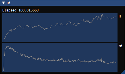
To evaluate how well this is working, we want to check two things
- Do we preserve the wave reasonably well?
- Are the constraint errors bounded?
This is for a 128^3 sized simulation, a timestep of 0.001, and with video capturing software that can’t handle sRGB correctly. $k_m$ for the momentum constraint damping is set to $0.025$. The precision of variables in memory is 32-bit floats, and 16-bit25 floats are used for precalculated derivatives. We can see here that the momentum constraint errors are decreasing, the hamiltonian constraint errors don’t blow up horribly, and the nature of the wave we’re simulating is preserved - though it does slowly dissipate. Oddly, we do way better here than we should do, according to this paper the bssn formalism should have failed with unbounded constraint errors - but I won’t complain too much about things going well
Performance here is excellent - with diagnostics (which are not at all optimised) disabled, it takes 16ms/tick (on a 6700xt), and 29ms/tick with them enabled. This is very competitive with a different simulator I wrote for binary black hole collisions, so we’re in a good spot for the future
All in all: Great success
Next time
This article is fairly dry with unexciting results - for good reason. If we tried to cram black hole collisions in here, it’d be even longer and I suspect no amount of cat pictures would save us from the sheer length of this piece. Luckily, future articles should be a lot simpler than this one - we’ve gotten the bulk of the technical work out of the way, which leaves us free to implement cool stuff
If you have any questions about this, or you get stuck/lost - please feel free to contact me. This is one of those areas that’s brutally difficult to get into as there are no guides, and I’m very happy to help people implement stuff
Until then:

Discussion: Conformal factors
There are actually three conformal variables I know of which are in use:
\[\begin{align} \tilde{\gamma}_{ij} &= e^{-4\phi} \gamma_{ij}\\ \tilde{\gamma}_{ij} &= \chi \gamma_{ij}\\ \tilde{\gamma}_{ij} &= W^2 \gamma_{ij}\\ \end{align}\]All defining the same conformal metric. The definition of the conformal variables in these schemes is as follows:
\[\begin{align} \phi &= \frac{1}{12} ln(det(\gamma))\\ \chi &= det(\gamma)^{-1/3}\\ W &= det(\gamma)^{-1/6}\\ \end{align}\]With this definition, the determinant of our conformal metric tensor is always $\tilde{\gamma} = 1$. The inverse of the metric tensor follows a similar relation:
\[\begin{align} e^{-4\phi} &\tilde{\gamma}^{ij} &= \gamma^{ij}\\ \chi &\tilde{\gamma}^{ij} &= \gamma^{ij}\\ W^2 &\tilde{\gamma}^{ij} &= \gamma^{ij}\\ \end{align}\]$\phi$26: This was the first to be used, but it tends to infinity at a black hole’s singularity which makes it not ideal - and appears to be falling out of use.
$\chi$: This version tends to 0 at the singularity and in general behaves much better than the $\phi$ version - it is relatively widespread in more modern code.
$W^2$: Ostensibly it has better convergence27 than $\chi$, but the really neat part about it is that renders the equations of motion of BSSN in a much less singular form. It also does not suffer from some of the issues that $\chi$ has, like unphysical negative values
Because of this, the $W^2$ formalism is clearly the best choice for us. Do note that some papers interchange notation here unfortunately, and eg $\phi$ and $\chi$ are sometimes used to mean any conformal factor
Discussion: Algebraic Constraint Enforcement
Here I’ll run through some alternatives you might find in the literature for managing the algebraic constraints, though they’re less common
Damping
This method involves damping the algebraic constraints over time. This paper contains a discussion of the idea (before 26), and you can use the specific form provided by this paper in the appendix. This means that the evolution equations are modified as follows:
\[\begin{align} \partial_t \tilde{\gamma}_{ij} &= \partial_t \tilde{\gamma}_{ij} + k_1\alpha \tilde{\gamma}_{ij} \mathcal{S}\\ \partial_t \tilde{A}_{ij} &= \partial_t \tilde{A}_{ij} + k_2\alpha \tilde{\gamma}_{ij} \mathcal{A} \end{align}\]Where $k_1$ < 0, $k_2$ < 0, and the constraints are evaluated from the relevant constraint expressions
Note that because this only damps the $\mathcal{A}$ constraint instead of eliminating it, you must also modify the evolution equation for $\tilde{\gamma}_{ij}$ as follows, to prevent everything from blowing up:
\[\partial_t \tilde{\gamma}_{ij} = \beta^m \partial_m \tilde{\gamma}_{ij}+ 2 \tilde{\gamma}_{m(i} \partial_{j)} \beta^m - \frac{2}{3} \tilde{\gamma}_{ij} \partial_m \beta^m - 2 \alpha \tilde{A}^{TF}_{ij} \\\]This works well, though you must be careful about your choice of damping factor. Too low and constraint errors pile up, too high and you overcorrect - causing errors
Solving
The constraints can also be seen to reduce the number of free components for \(\tilde{\gamma}_{ij}\) and \(\tilde{A}_{ij}\) from 6 to 5, and instead of enforcing or damping the constraints, you can use them to solve for one of the components instead. For more discussion on this approach, please see this paper (36-37)
Discussion: Boundary conditions + Derivatives Performance
Modulo operator
Do be aware that I discovered a pretty sizeable performance bug/compiler limitation when implementing this, where modulo operations are not optimised (even by a constant power of 2!) - which ate nearly all the runtime, so use branches instead
Second derivatives
When calculating second derivatives, while you could directly apply a 2d stencil, it is much more efficient to first calculate the first derivatives, store them somewhere, and then calculate the second derivatives from those stored derivatives (by taking the first derivative28 of them). This means that you should only precalculate 1st derivatives for variables for which we take second derivatives, which are the following:
\[\tilde{\gamma}_{ij}, \alpha, \beta^i, W\]Second derivative performance tricks
Second derivatives commute. This means that $\partial_i \partial_j == \partial_j \partial_i$. This is also true for the second covariant derivative of a scalar - though only in that circumstance for covariant derivatives. This brings up a good opportunity for performance improvements - when calculating partial derivatives, consider reordering them so that you lopsidedly differentiate in one direction
That is to say, consider implementing: $\partial_{min(i, j)} \partial_{max(i, j)}$ as a general second order differentiation system. This is good for cache (repeatedly accessing the same memory), increasing the amount of eliminateable duplicate code, and ensuring that we maximise the amount we differentiate in the $_0$th direction, which is the fastest due to memory layout
Eg, if we precalculate the first derivative $\partial_i \alpha$, calculating $\partial_0 \partial_i \alpha$ will always be faster than calculating $\partial_i \partial_0 \alpha$. Partly because of memory layout (differentiating in the x direction is virtually free, as it is very cache friendly), and partly because if we always do this, we improve our cache hit rate. This is worth about a 20% performance bump29:
Where exactly is the boundary?
One fairly key point that may not immediately obvious is how to lay out your initial conditions in a periodic system vs a non periodic system. Lets say we have a physical width of 1, and a grid width of 128, with periodic initial conditions. We want grid cell 0, and grid cell 128 + 1 (ie the wrapped coordinate) to both exactly represent the same point. This means that grid cell 0 exists at at the coordinate 0, and the virtual cell 129 exists at the coordinate 1. The scale is 1/128
In a non periodic system, things are different - I normally use odd grid sizes so that there’s a central grid cell. So given a size of 127, the centre is (127 - 1)/2. We want the rightmost grid cell to map to the coordinate 1, and the leftmost gridcell to map to the coordinate 0. This is notably different to the periodic initial conditions setup, as the coordinate distance between our cells is now structurally not the same - its 1/(127-1)
Discussion: Gauge conditions
To chop down on unnecessary side tracking, I’m putting some other examples of gauge conditions here at the end
Geodesic slicing
\[\alpha = 1, \beta^i = 0\]Lapse ($\alpha$)
Harmonic slicing
Ref30
\[\partial_t \alpha = - \alpha^2 K + \beta^m \partial_m \alpha\]1+log slicing
Ref31
\[\partial_t \alpha = - 2 \alpha K + \beta^m \partial_m \alpha\]Shift ($\beta^i$)
Zero shift
\[\beta^i = 0\]Gamma driver (sometimes called Gamma freezing)
Ref32
So called because it drives $\partial_t\tilde{\Gamma} = 0$
\[\partial_t \beta^i = \frac{3}{4} \tilde{\Gamma}^i + \beta^j \partial_j \beta^i - n \beta^i\]$n$ is a damping parameter, that is generally set to $2$, or $2M$ where $M$ is the mass of whatever you have in your spacetime
The alternative form of this gauge condition is:
\[\begin{align} \partial_t \beta^i &= \beta^m \partial_m \beta^i + \frac{3}{4} B^i\\ \partial_t B^i &= \beta^m \partial_m B^i + \partial_t \tilde{\Gamma}^i - \beta^m \partial_m \tilde{\Gamma}^i - n B^i \end{align}\]As far as I know, nobody has ever really found a compelling reason to use this form of the gamma driver gauge condition (plus, it is slower and requires more memory), so I’m really only mentioning it because it shows up in the literature. The single variable form of the gamma driver condition is the integrated form of the two-variable expression
Alternate forms
The self advection terms for both lapse and shift are optional and often are disabled, ie $\beta^m \partial_m \alpha$ and $\beta^j \partial_j \beta^i$
Gauge condition summary
In the test we will be looking at today, the time coordinate is defined as being harmonic, which is why we’re sticking with it. The binary black hole gauge (often called the moving puncture gauge) is 1+log + Gamma driver, and will be used virtually exclusively in future articles
One important feature of gauge conditions is that they ideally tend towards $\alpha = 1$, and $\beta^i = 0$ as you move towards flat spacetime. This simplifies things like gravitational wave extraction, or mass calculation down the line
-
You’ll need 8+ GB of vram for future bbh collisions, though you can get away with minimal specs for this article. This was written and tested on a 6700xt, but previous work was on an r9 390. Any OpenCL 1.2 compatible device will work here, though I do use 64-bit atomics for accumulating diagnostics ↩
-
This statement comes with caveats about GR being a coordinate free theory. The formalism we’re going to get into - BSSN - is not a coordinate free theory, and coordinate free versions of it in general appear to be less numerically stable. For this reason, we’re not going to dip into coordinate free territory at all ↩
-
That said, the ADM formalism is more restricted in what it can represent. Notably, our spacetime’s topology cannot change, which means that the formation of wormholes cannot be simulated in the ADM formalism ↩
-
These are also often frequently labelled $N$, for the lapse, and $N^i$, for the shift ↩ ↩2
-
See Introduction to the ADM Formalism page 3. Frankly this document gives a better description of the ADM formalism than I ever could ↩ ↩2
-
If you’re coming into this with no knowledge of GR, a metric tensor is used to measure distances, and angles, and defines the warping of spacetime. $\gamma_{ij}$ is used on this 3d space, whereas a 4-metric called $g_{\mu\nu}$ is used on a 4d spacetime ↩
-
https://arxiv.org/pdf/gr-qc/0604035 (5). There are other forms of these equations, but these are the most common form in numerical relativity ↩
-
Its not true that the ADM formalism is useless in general, but if you want to simulate binary black hole collisions, then it won’t work. We’re also going to get into neutron stars collapsing into black holes, which is even less numerically stable ↩
-
https://arxiv.org/pdf/0707.0339 this paper contains a lot of useful details, but the short version is that the BSSN equations are a partially constrained evolution system33, and managing the constraints is critical to a correct evolution scheme ↩
-
$\tilde{\Gamma}^i_{jk}$ are the conformal christoffel symbols of the second kind, calculated in the usual fashion from $\tilde{\gamma_{ij}}$. $\Gamma^i_{jk}$ are the christoffel symbols associated with $\gamma_{ij}$ ↩
-
For a lot of detail on why and how the christoffel symbol exists, see this page 47 onwards, and here page 58 onwards ↩
-
Technically the conformal metric is a tensor density with weight $-\frac{2}{3}$ ↩
-
There’s no real single form of the BSSN equations. I’ve copied these from slide 37, and taken the expression for the curvature tensor from here (12). Because the slides use a different conformal decomposition, I’ve performed the substitution manually, as the $W^2$ formalism tends to be used in newer non bssn formalisms. There may be a better reference for $W^2$, but I don’t have one off-hand as this is the first time I’ve implemented $W^2$ entirely from scratch as the root conformal variable, rather than ad-hoc’ing it into an existing $\chi$ formalism ↩
-
Note that for some scalar $A$, $(AQ)^{TF} == A(Q^{TF})$, and it does not matter if you use the conformal metric, or the non conformal metric as the metric tensor here - the conformal factor cancels out. This is also sometimes notated $Q_{\langle ij \rangle}$ ↩
-
This footnote could (and likely will) be an entire article in the future, where we’ll test out dozens of modifications. Until then, consider checking out this, this, and the ccz4 paper (a similar, constraint damped formalism) for more information. There’s a lot of decent analysis spread over the literature ↩
-
The Einstein toolkit references Global Atmospheric Research Programme Publication Series no. 10, which can be found on the World Meteorological Organization e-Library. Many thanks to Miro Palmu (website link) for finding this reference. The original Kreiss and Oliger (1972) paper is also available here ↩
-
It is not clear to me when people refer to the order of kreiss-oliger dissipation if they mean the derivatives, or $p$. eg in this paper, B.4 is called 4th order kreiss-oliger, whereas the cactus toolkit contradicts that definition ↩
-
Note that its common to use Newton-Raphson or a full root finding method here for solving implicit equations, and I’ve had nothing but poor results. The issue is that it is not a massively stable algorithm, and the complexity of evaluating a Newton-Raphson iteration outweighs the increase in convergence when dealing with a small number of iterations (eg 2-3 here). Fixed point iteration can be directly sped up by rearranging it as a relaxation problem, and then successively over relaxing ↩
-
If you’re unfamiliar with this syntax, its called a line element. I go into this in a lot more detail in the Schwarzschild article ↩
-
Where I found $K_{ij}$ from is here 4-19a, although its a bit of a random source ↩
-
In general, the order of convergence dictates the rate at which our algorithm improves the answer, when eg increasing our grid resolution ↩
-
Technically, as $\alpha$ is expected to tend to 0 faster than $W$ tends to 0, the quantity $\frac{\alpha}{W}$ is considered regular. In practice, clamping the conformal factor appears to be the accepted technique, though alarmingly I’ve found that the exact clamp value can make a large difference to your simulation ↩
-
This might seem a slightly surprising choice in software intended to be scientific, but amazingly enough it has very little bearing on the evolution results. It is however easily swappable for exactly this reason, to facilitate testing - and I have extensively tested this with BBH sims. Given that the range of derivatives is inherently small in a smooth solution, fixed point might provide better results than 16-bit floats. The main advantage of 16-bit floats is the reduced memory usage, which will enable us to simulate higher resolution spacetimes in the future. In general, the appropriate storage format for these problems is an interesting question, as floating point wastes a huge amount of precision when we have variables with a known range ↩
-
There wasn’t a good place to put this footnote in, here’s an example of the equations and definitions with a phi scheme Numerical experiments of adjusted BSSN systems for controlling constraint violations ↩
-
See High-spin binary black hole mergers for this line of reasoning ↩
-
I’ve said the word derivative too many times. I’m going to go pet my cat ↩
-
This performance increase is difficult to interpret. In this test case, we use slightly more vGPRs (vector general purpose registers, what you might think of as a traditional cpu register), but significantly reduce our code instruction footprint from 35KB (over the icache size of 32KB), to below our maximum cache size (AMD don’t report it annoyingly). This reduces icache stalls, and appears to be very related to the performance increase. Its a big win, as there’s 0% chance of us hitting a better vGPR budget34 (as we’re in the low 200s) ↩
-
Gauge conditions for long-term numerical black hole evolutions without excision 33 + 34 ↩
-
How to move a black hole without excision: gauge conditions for the numerical evolution of a moving puncture 26 ↩
-
If you’re unfamiliar, the number of threads we can execute on a GPU simultaneously is limited by the number of registers we use, and is known as occupancy (high occupancy = more threads executing). Traditional reasoning is that high occupancy = good as it hides memory latency, although low occupancy can have have performance benefits in some circumstances. GPUs are a pain ↩