Numerical Relativity 103: Raytracing numerical spacetimes
Hi! Today we’re going to look at raytracing numerical spacetimes. We’re going to explore two things:
- The ADM geodesic equations to produce a fast approximate rendering on a single slice through spacetime
- The regular geodesic equation to accurately raytrace inspiralling binary black holes
Along the way, I’ll present a modified form of the Verlet algorithm, which is particularly well suited for integrating these kinds of problems. At the end of the article, we’ll have rendered out this:
I’d highly recommend reading this introduction to geodesics in general relativity as it gives a good structure on how these simulations work, and this article about tetrads describes the process for constructing the initial conditions
If you’re looking for someone with a lot of enthusiasm for GPU programming, and who’d rather love to do a PhD in numerical relativity - please give me a shout! 1
The code for this article is available over here as always

What’s the general structure of what we’ll be doing?
Like any traditional raytracer, there are three parts:
- Initial conditions
- Integration
- Termination conditions
In general, a raytracer of this form involves setting up light rays that travel backwards in time, and tracking their movement around a grid - where our acceleration is a function of the grid variables. We’ll be checking if our rays have probably2 hit a black hole, or if they’ve escaped into the wider universe
We’ll either be keeping rays on a single slice for debugging, or allowing rays to traverse multiple slices for accurate rendering
In general, the initial conditions and termination conditions are no different in a numerical simulation compared to an analytic system, and are fully described in the articles linked at the beginning. I’ll be largely be dealing with the integration step as a result
Recap
What are geodesics?
In general relativity, geodesics represent paths through spacetime. They come in three types:
- Timelike, representing the paths of observers and massive particles
- Null (or lightlike), representing the paths of massless particles like light
- Spacelike, representing paths that cannot be traversed causally
In general, we’re only interested in timelike and null geodesics. Everything in this article is applicable to both of these kinds of geodesics unless otherwise mentioned - though we’re not going to simulate timelike geodesics today
Geodesics have two properties:
- A 4-position, which we’ll notate as $x^\mu$
- A 4-velocity, which we’ll notate as $\frac{dx^\mu}{d\lambda}$. Note that this velocity is the derivative of the position $x^\mu$ with respect to either an affine parameter $d\lambda$ (sometimes called $ds$), or coordinate time $dt$. We’ll be exclusively sticking with the former, to avoid confusion
Greek indices run from $[0,4)$ and represent quantities on the 4d spacetime. Latin indices run from $[1,4)$, and generally represent quantities on the 3d hypersurface
The ADM formalism
The ADM formalism is the process of taking a 4-metric $g_{\mu\nu}$, and splitting it up into a series of 3d slices (called a foliation). Each 3d slice has a number of variables associated with it: $\gamma_{ij},\;K_{ij},\;\alpha,\;\beta^i$. I’ll list a table of all the relevant conversions and definitions at the end of this article. The main one to remember is that $\gamma_{ij}$ is the metric tensor on the current 3d slice (the ‘induced’ metric)
Unlike previous articles, we’ll be barely dealing with the BSSN formalism (an offshoot of ADM) at all. I’ll be mentioning it in passing, but we’ll use it solely to construct the relevant ADM quantities
The ADM geodesic equation
Today we’re primarily going to be dealing with the paper 3+1 geodesic equation and images in numerical spacetimes, and discussing some of the implications. Lets get into it
Initial conditions
The way we set up initial conditions is exactly as described in previous articles, with no changes. The sole difference is that we build the metric tensor $g_{\mu\nu}$ from the ADM components ($\gamma_{ij},\; \alpha,\; \beta^i$), rather than having a metric analytically. You’ll want to implement trilinear interpolation on the fields, if your camera lives on a non integer coordinate
Because there’s nothing special here, lets assume that we have a geodesic (either null, or timelike), with a position $x^\mu$ and a velocity $\frac{dx^\mu}{d\lambda}$. We’re primarily looking to find a velocity $V^i$ on our 3d slice - the projection of the 4-velocity
This paper requires us to calculate the 4-momentum of our geodesic, $p^\mu$. This is slightly different for timelike, and null geodesics:
| Type | Relation |
|---|---|
| Timelike | \(p^\mu = m \frac{dx^\mu}{d\tau}\)3 |
| Null | \(p^\mu = \frac{dx^\mu}{d\lambda}\) |
Where $m$ is the rest mass, and we’ve set $d\lambda = d\tau$ (the proper time) for timelike geodesics. For null geodesics, the 4-momentum is equivalent to rescaling the 4-velocity, which has no effect on the path (as rescaling a null geodesic is equivalent to a change in the affine parameter)
Next up, we want to find the 3-velocity of the ray, which is the projection of our 4-velocity on the 3-surface - ie we’re translating from GR to ADM. To do this, simply apply (8), and solve for $V^\mu$:
\[V^\mu = \frac{p^\mu}{E} - \mathcal{n}^\mu\]Where:
- $E = -p_\mu \mathcal{n}^\mu$4
- $\mathcal{n}^\mu = (\frac{1}{\alpha}, -\frac{\beta^0}{\alpha}, -\frac{\beta^1}{\alpha}, -\frac{\beta^2}{\alpha})$
This procedure breaks up the momentum $p^\mu$ into two parts:
- A component $V^i$ tangent to our hypersurface. This means $V^\mu$ has no component in the timelike direction ($\mathcal{n}_\mu V^\mu = 0$, and $V^0 = 0$)
- A component which is normal to the hypersurface, ie pointing forwards in a timelike direction. Finding the evolution of $V^i$ in the normal direction ($\mathcal{n}^\mu$) gives us the geodesic equations
For null geodesics, $V_i V^i = 1$, and for timelike geodesics, $V_i V^i < 1$. Indices are raised and lowered with $\gamma_{ij}$ as normal
So, for tracing a geodesic in the ADM formalism, we have two things at the end of our initial conditions:
- A 3-position, which we’ve called $x^i$, and this paper calls $X^i$. This is just the last three coordinates of $x^\mu$
- A 3-velocity $V^i$, which is the projection our 4-velocity onto our local hypersurface. It is important to note that this is not the derivative of $x^i$
Implementation: Projection
Because the initial conditions for ADM are the same as the non ADM version but with a projection step, I mix together both into one common routine. There’s nothing too exciting in here
geodesic my_geodesic = <setup>

v2i out_dim = screen_sizel.get();
v2i out_pos = {x, y};

//use the format (t, x, y, z) for both formalisms
as_ref(positions_out[out_pos, out_dim]) = my_geodesic.position;

//adm formalism: do the projection
if_e(is_adm.get() == 1, [&]{
    adm_variables init_adm = admf_at(grid_position, dim.get(), in);

    tensor<valuef, 4> normal = get_adm_hypersurface_normal_raised(init_adm.gA, init_adm.gB);
    tensor<valuef, 4> normal_lowered = get_adm_hypersurface_normal_lowered(init_adm.gA);

    //energy
    valuef E = -sum_multiply(my_geodesic.velocity, normal_lowered);

    //projection
    tensor<valuef, 4> adm_velocity = ((my_geodesic.velocity / E) - normal);

    as_ref(velocities_out[out_pos, out_dim]) = adm_velocity;
});

//no projection necessary in the non adm case
if_e(is_adm.get() == 0, [&]{
    as_ref(velocities_out[out_pos, out_dim]) = my_geodesic.velocity;
});
As usual I’m just pulling out the interesting bits, and the code for this is available over here
Implementation: BSSN -> ADM
To construct the ADM variables from the BSSN variables, I use a standard trilinear interpolation:
adm_variables admf_at(v3f pos, v3i dim, bssn_args_mem<buffer<valuef>> in)
{
    using namespace single_source;

    adm_variables out;

    auto cY_at = [&](v3i pos) {
        return bssn_at(pos, dim, in).cY;
    };

    auto W_at = [&](v3i pos) {
        return bssn_at(pos, dim, in).W;
    };

    auto cA_at = [&](v3i pos) {
        return bssn_at(pos, dim, in).cA;
    };

    auto K_at = [&](v3i pos) {
        return bssn_at(pos, dim, in).K;
    };

    auto gA_at = [&](v3i pos) {
        return bssn_at(pos, dim, in).gA;
    };

    auto gB_at = [&](v3i pos) {
        return bssn_at(pos, dim, in).gB;
    };

    auto cY = function_trilinear(cY_at, pos);
    auto cA = function_trilinear(cA_at, pos);
    auto W = function_trilinear(W_at, pos);
    auto K = function_trilinear(K_at, pos);
    auto gA = function_trilinear(gA_at, pos);
    auto gB = function_trilinear(gB_at, pos);

    out.Yij.from_tensor(cY.to_tensor() / (W*W));
    out.Kij = (cA + cY.to_tensor() * (K/3.f)) / (W*W);
    out.gA = gA;
    out.gB = gB;

    pin(out.Yij);
    pin(out.Kij);
    pin(out.gA);
    pin(out.gB);

    return out;
}
A slight wrinkle: Photons going backwards in time
The standard in these simulations it to raytrace light rays backwards in time. If you’re doing this (which we are), you’ll note that we have no component in the timelike direction for $V^i$. The slightly odd thing to realise is that the timestep becomes negative when performing the integration, as we’re quite literally doing negative steps through coordinate time
Evolution equations
The evolution equations for our system are given by (28a) and (28b):
\[\begin{align} \frac{dX^i}{dt} &= \alpha V^i - \beta ^i \\ \frac{dV^i}{dt} &= \alpha V^j (V^i (\partial_j \ln(\alpha) - K_{ij} V^k) + 2 K^i_j - ^3\Gamma^i_{jk} V^k) \\&- \gamma^{ij} \partial_j \alpha - V^j \partial_j \beta^i \\ \end{align}\]Where $^3 \Gamma^i_{jk}$ are the Christoffel symbols associated with $\gamma_{ij}$. I’ve converted this papers notation to ours, ie $\alpha = N$
The only modifications we’ll make are as follows:
- $\frac{\partial_j \alpha}{\alpha}$ is easier to calculate than $\partial_j \ln(\alpha)$
- For null geodesics, enforcing $V_i V^i = 1$ by rescaling the length improves accuracy
- The Christoffel symbols can be calculated from the BSSN variables directly, eg see (A3)
That is to say:
\[\Gamma^i_{jk} = \tilde{\Gamma}^i_{jk} - \frac{\delta^i_j \partial_k W + \delta^i_k \partial_j W - \tilde{\gamma}_{jk} \partial^i W}{W}\]Where $\delta^i_j$ is the kronecker delta, and \(\partial^i = \tilde{\gamma}^{ij} \partial_j\)
Approximate rendering on a single slice
With the evolution equations in hand, we’ll want to get to implementing. We’re going to be using this just to produce a debug visualisation on a single slice. The reason why we won’t be using this for accurate raytracing is that its much less memory efficient - which is something that will become apparent when we get there
The first thing we need before we get started however, is to pick an integrator. Its important to pick a good choice here, as it’ll govern our performance
Verlet
Euler integration is not very good for these problems, even if it does tend to be the default integrator for many problems. It has poor performance for its accuracy, and additionally it isn’t symplectic. This means that a ray’s energy tends to diverge, and its not a great choice in general
We can pick a much better algorithm: Verlet. First off, we’ll take a look at the basic Verlet algorithm for this problem, and then tweak it to improve performance
Verlet for non separable hamiltonians
Wikipedia lists a form of the velocity Verlet algorithm which isn’t super helpful to us. Unfortunately, we have two problems:
- The velocity $V^i$ is not directly the velocity of $X^i$
- The acceleration is a function of the position and velocity
These are both really the same problem: what we have is known as a non separable hamiltonian. This means our equations are of the form:
\[\begin{align} \dot{q} &= g(q, v)\\ \dot{v} &= f(q, v) \end{align}\]We need a slightly more general form of Verlet integration to combat this. A more useful form is defined by (1.24) here - which is applicable to our problem
The choice of which function is $g$ or $f$ determines which variable is $q$ or $v$. In our case, we’ll pick the following convention5:
- $g(q, v) = dX(x(t), v(t))$
- $f(q, v) = dV(x(t), v(t))$
Where $q$ is the position $X^i$, $v$ is the velocity $V^i$, $g$ is $dX$, and $f$ is $dV$. This gives the following integration scheme:
\[\begin{align} V_{n+\frac{1}{2}} &= V_n + \frac{h}{2}dV(X_n, V_{n+\frac{1}{2}})\\ X_{n+1} &= X_n + \frac{h}{2}(dX(X_n, V_{n+\frac{1}{2}}) + dX(X_{n+1}, V_{n+\frac{1}{2}}))\\ V_{n+1} &= V_{n+\frac{1}{2}} + \frac{h}{2} dV(X_{n+1}, V_{n+\frac{1}{2}})\\ \end{align}\]Where $h$ is the timestep, and $n$ is the iteration variable. You might notice that these equations are implicit, ie we have terms which are on both sides of the equation. Solving these equations efficiently might seem prohibitively expensive right off the bat, especially compared to just lowering the timestep with a simple Euler scheme. Luckily the problem we’re trying to solve allows us to make some simplifications and assumptions, based on its characteristics:
- $dV(X, V)$ is expensive to evaluate for different values of $X$, but cheap to evaluate for different values of $V$
- $dV(X, V)$ is only weakly dependent on the value of $V$, ie $dV(X, V + \epsilon) \approx dV(X, V)$
- $dX(X, V)$ is cheap to evaluate
- The underlying problem is not numerically unstable, and is well conditioned
So, lets do some approximating and rewrite these equations in an explicit form:
\[\begin{align} V_{n+\frac{1}{2}} &= V_n + \frac{h}{2}dV(X_n, V_n)\\ \bar{X}_{n+1} &= X_n + h \; dX(X_n, V_n)\\ X_{n+1} &= X_n + \frac{h}{2}(dX(X_n, V_{n+\frac{1}{2}}) + dX(\bar{X}_{n+1}, V_{n+\frac{1}{2}}))\\ V_{n+1} &= V_{n+\frac{1}{2}} + \frac{h}{2} dV(X_{n+1}, V_{n+\frac{1}{2}})\\ \end{align}\]I’ve replaced $\frac{h}{2}dV(X_n, V_{n+\frac{1}{2}})$ with $\frac{h}{2}dV(X_n, V_n)$6, and approximated the initial value of $X_{n+1}$ with an Euler guess. While in theory this reduces the stability and accuracy of the integrator, in practice due to the nature of the problem we’re trying to solve, this works extremely well
The last thing we need to do is solve the evaluation of $dV$ with different values of $X$ - we can straightforwardly rework these equations to only evaluate $dV$ for a single $X$. To do this, we’ll split this up into two phases: initialisation, and then our iteration step. I’ll also be relabling $h$ as $h_n$, as the timestep is dynamic:
Initialisation:
\[\begin{align} V_{\frac{1}{2}} &= V_0 + \frac{h_0}{2}dV(X_0, V_0)\\ \bar{X}_{1} &= X_0 + h_0 \; dX(X_0, V_0)\\ X_{1} &= X_0 + \frac{h_0}{2}(dX(X_0, V_{0+\frac{1}{2}}) + dX(\bar{X}_{1}, V_{\frac{1}{2}}))\\ \end{align}\]Iteration, starting at $n=1$:
\[\begin{align} V_{n} &= V_{n-\frac{1}{2}} + \frac{h_{n-1}}{2} dV(X_{n}, V_{n-\frac{1}{2}})\\ V_{n+\frac{1}{2}} &= V_n + \frac{h_n}{2}dV(X_n, V_n)\\ \bar{X}_{n+1} &= X_n + h_n \; dX(X_n, V_n)\\ X_{n+1} &= X_n + \frac{h_n}{2}(dX(X_n, V_{n+\frac{1}{2}}) + dX(\bar{X}_{n+1}, V_{n+\frac{1}{2}}))\\ \end{align}\]We now only evaluate $dV$ for the same $X_n$ within an iteration, which is roughly a 2x performance speedup. One oddity here is that the velocity iteration variable becomes $V_{n+\frac{1}{2}}$, and there’s no need to store $V_n$. $h_n$ is also promoted to a variable as well, as its value is carried across loops

Implementating Verlet
This form of Verlet integration is well suited for both the ADM equations, and the regular geodesic equation. Because of this, I decided to finally implement a generic Verlet integrator that I can reuse:
template<typename T, int N>
struct verlet_context
{
    tensor<mut<T>, N> position;
    mut<T> ds_m;
    tensor<mut<T>, N> last_v_half;
    tensor<mut<T>, N> velocity;

    template<typename dX, typename dV, typename dS, typename State>
    void start(const tensor<T, N>& X_in, const tensor<T, N>& V_in, dX&& get_dX, dV&& get_dV, dS&& get_dS, State&& get_state)
    {
        using namespace single_source;

        position = declare_mut_e(X_in);
        velocity = declare_mut_e(V_in);

        auto x_0 = declare_e(X_in);
        auto v_0 = declare_e(V_in);

        auto st = get_state(x_0);

        auto acceleration = get_dV(x_0, v_0, st);
        pin(acceleration);

        auto ds = get_dS(x_0, v_0, acceleration, st);
        pin(ds);

        auto v_half = v_0 + 0.5f * ds * get_dV(x_0, v_0, st);

        auto x_full_approx = x_0 + ds * get_dX(x_0, v_0, st);
        auto st_full_approx = get_state(x_full_approx);

        auto x_full = x_0 + 0.5f * ds * (get_dX(x_0, v_half, st) + get_dX(x_full_approx, v_half, st_full_approx));

        last_v_half = declare_mut_e(v_half);
        ds_m = declare_mut_e(ds);
        as_ref(position) = x_full;
    }

    template<typename dX, typename dV, typename dS, typename State>
    auto next(dX&& get_dX, dV&& get_dV, dS&& get_dS, State&& get_state, auto&& enforce_velocity_constraint)
    {
        using namespace single_source;

        auto x_n = declare_e(position);
        auto v_nhalf = declare_e(last_v_half);
        auto ds_n1 = declare_e(ds_m);

        auto st = get_state(x_n);

        auto v_n = v_nhalf + 0.5f * ds_n1 * get_dV(x_n, v_nhalf, st);

        v_n = enforce_velocity_constraint(v_n, st);
        pin(v_n);

        auto acceleration = get_dV(x_n, v_n, st);
        pin(acceleration);

        auto ds = get_dS(x_n, v_n, acceleration, st);
        pin(ds);

        auto v_half = v_n + 0.5f * ds * get_dV(x_n, v_n, st);

        auto x_full_approx = x_n + ds * get_dX(x_n, v_n, st);
        auto st_full_approx = get_state(x_full_approx);

        auto x_full = x_n + 0.5f * ds * (get_dX(x_n, v_half, st) + get_dX(x_full_approx, v_half, st_full_approx));

        as_ref(position) = x_full;
        as_ref(last_v_half) = v_half;
        as_ref(ds_m) = ds;
        //I only update this for rasterisation reasons
        as_ref(velocity) = v_half;

        //this is returned so we can use it for termination conditions
        return get_dX(x_n, v_half, st);
    }
};
Here, the timestep is called $ds$, and is assumed to be some function of position, velocity, and acceleration. We also carry a state around, which is used to avoid re-evaluating the same expressions repeatedly
With all of this together, Verlet is about 3-5x better than Euler in terms of step size, for a similar cost of evaluating the equations - as we only evaluate the expensive part of $dV$ once per iteration. It does come with a register and compute penalty, but its worth the tradeoff
Implementing The ADM geodesic equations
Timestepping
The timestepping here is pretty simple. $W$ is assumed to be a good measure of how close we are to a black hole, and $W^2$ turns out to be a reasonably good variable for determining the step size:
valuef get_ct_timestep(valuef W)
{
    float X_far = 0.9f;
    float X_near = 0.6f;

    valuef X = W*W;

    valuef my_fraction = (X - X_near) / (X_far - X_near);

    my_fraction = clamp(my_fraction, 0.f, 1.f);

    return mix(valuef(0.1f), valuef(1.f), my_fraction);
}
These constants are a bit arbitrary, but work fine. If you come up with a better scheme than this, please do let me know
Raytracing
The basic form of the raytracing scheme is as follows:
void trace3(execution_context& ectx, literal<v2i> screen_sizel,
            literal<v4f> camera_quat,
            buffer_mut<v4f> positions, buffer_mut<v4f> velocities,
            buffer_mut<valuei> results, buffer_mut<valuef> zshift,
            literal<v3i> dim,
            literal<valuef> scale,
            bssn_args_mem<buffer<valuef>> in,
            bssn_derivatives_mem<buffer<derivative_t>> derivatives)
{
    using namespace single_source;

    valuei x = value_impl::get_global_id(0);
    valuei y = value_impl::get_global_id(1);

    //get_global_id() is not a const function, so assign it to an unnamed variable to avoid compilers repeatedly evaluating it
    pin(x);
    pin(y);

    v2i screen_size = screen_sizel.get();

    //terminate if we're out of bounds
    if_e(y >= screen_size.y(), [&] {
        return_e();
    });

    if_e(x >= screen_size.x(), [&] {
        return_e();
    });

    v2i screen_position = {x, y};

    v3f pos_in = declare_e(positions[screen_position, screen_size]).yzw();
    v3f vel_in = declare_e(velocities[screen_position, screen_size]).yzw();

    mut<valuei> result = declare_mut_e(valuei(2));

    <get_dX, get_dV, get_dS, get_state, and fix_velocity go here>

    verlet_context<valuef, 3> ctx;
    ctx.start(pos_in, vel_in, get_dX, get_dV, get_dS, get_state);

    mut<valuei> idx = declare_mut_e("i", valuei(0));

    for_e(idx < 512, assign_b(idx, idx + 1), [&]
    {
        v3f cposition = declare_e(ctx.position);
        v3f cvelocity = declare_e(ctx.velocity);

        valuef radius_sq = dot(cposition, cposition);

        //terminate if we're out of the sim
        if_e(radius_sq > UNIVERSE_SIZE*UNIVERSE_SIZE, [&] {
            as_ref(result) = valuei(1);
            break_e();
        });

        //terminate if our rays become non finite
        if_e(!isfinite(cvelocity.x()) || !isfinite(cvelocity.y()) || !isfinite(cvelocity.z()), [&]{
            as_ref(result) = valuei(0);
            break_e();
        });

        v3f diff = ctx.next(get_dX, get_dV, get_dS, get_state, fix_velocity);

        //terminate if the movement of our ray through coordinate space becomes approximately zero, its likely hit an event horizon
        if_e(diff.squared_length() < 0.1f * 0.1f, [&]
        {
            as_ref(result) = valuei(0);
            break_e();
        });
    });

    v3f final_position = declare_e(ctx.position);
    v3f final_velocity = declare_e(ctx.velocity);

    as_ref(positions[screen_position, screen_size]) = (v4f){0, final_position.x(), final_position.y(), final_position.z()};
    as_ref(velocities[screen_position, screen_size]) = (v4f){0, final_velocity.x(), final_velocity.y(), final_velocity.z()};
    as_ref(results[screen_position, screen_size]) = as_constant(result);
}
This is the loop structure without the update functions to give you a basic idea of what we’re looking at. The update functions are as follows:
//This enforces V_i V^i = 1
auto fix_velocity = [](v3f velocity, const trace3_state& args)
{
    auto cY = args.cY;
    auto W = args.W;

    auto Yij = cY / (W*W);

    valuef length_sq = dot(velocity, Yij.lower(velocity));
    valuef length = sqrt(fabs(length_sq));

    velocity = velocity / length;

    pin(velocity);

    return velocity;
};

auto get_dX = [](v3f position, v3f velocity, const trace3_state& args)
{
    v3f d_X = args.gA * velocity - args.gB;
    pin(d_X);

    return d_X;
};

auto get_dV = [&](v3f position, v3f velocity, const trace3_state& args)
{
    v3f grid_position = args.grid_position;

    auto dgA_at = [&](v3i pos) {
        bssn_derivatives derivs(pos, dim.get(), derivatives);
        return derivs.dgA;
    };

    auto dgB_at = [&](v3i pos) {
        bssn_derivatives derivs(pos, dim.get(), derivatives);
        return derivs.dgB;
    };

    auto dcY_at = [&](v3i pos) {
        bssn_derivatives derivs(pos, dim.get(), derivatives);
        return derivs.dcY;
    };

    auto dW_at = [&](v3i pos) {
        bssn_derivatives derivs(pos, dim.get(), derivatives);
        return derivs.dW;
    };

    //interpolate all the BSSN derivatives
    tensor<valuef, 3> dgA = function_trilinear(dgA_at, grid_position);
    tensor<valuef, 3, 3> dgB = function_trilinear(dgB_at, grid_position);
    tensor<valuef, 3, 3, 3> dcY = function_trilinear(dcY_at, grid_position);
    tensor<valuef, 3> dW = function_trilinear(dW_at, grid_position);

    pin(dgA);
    pin(dgB);
    pin(dcY);
    pin(dW);

    auto cY = args.cY;
    auto W = args.W;

    auto icY = cY.invert();
    pin(icY);

    ///inverse of the full adm metric
    auto iYij = icY * (W*W);

    //bssn christoffel symbols
    auto christoff2_cfl = christoffel_symbols_2(icY, dcY);
    pin(christoff2_cfl);

    //adm christoffel symbols
    auto christoff2 = get_full_christoffel2(W, dW, cY, icY, christoff2_cfl);
    pin(christoff2);

    tensor<valuef, 3> d_V;

    for(int i=0; i < 3; i++)
    {
        for(int j=0; j < 3; j++)
        {
            valuef kjvk = 0;

            for(int k=0; k < 3; k++)
            {
                kjvk += args.Kij[j, k] * velocity[k];
            }

            valuef christoffel_sum = 0;

            for(int k=0; k < 3; k++)
            {
                christoffel_sum += christoff2[i, j, k] * velocity[k];
            }

            valuef dlog_gA = dgA[j] / args.gA;

            d_V[i] += args.gA * velocity[j] * (velocity[i] * (dlog_gA - kjvk) + 2 * raise_index(args.Kij, iYij, 0)[i, j] - christoffel_sum)
                    - iYij[i, j] * dgA[j] - velocity[j] * dgB[j, i];

        }
    }

    return d_V;
};

auto get_dS = [&](v3f position, v3f velocity, v3f acceleration, const trace3_state& args)
{
    //3.5f chosen by hand
    return -3.5f * get_ct_timestep(args.W);
};

auto get_state = [&](v3f position) -> trace3_state
{
    trace3_state out;

    v3f grid_position = world_to_grid(position, dim.get(), scale.get());

    grid_position = clamp(grid_position, (v3f){3,3,3}, (v3f)dim.get() - (v3f){4,4,4});
    pin(grid_position);

    auto W = W_f_at(grid_position, dim.get(), in);
    auto cY = cY_f_at(grid_position, dim.get(), in);

    pin(W);
    pin(cY);

    adm_variables args = admf_at(grid_position, dim.get(), in);

    out.W = W;
    out.cY = cY;
    out.Kij = args.Kij;
    out.gA = args.gA;
    out.gB = args.gB;
    out.grid_position = grid_position;

    return out;
};
I take advantage here of the fact that the derivatives of the conformal variables are available from the main BSSN simulation, as well as the relation \(\gamma^{ij} = W^2 \tilde{\gamma}^{ij}\) (it’s faster to compute, given than \(\tilde{\gamma}_{ij}\) has a unit determinant)

Rendering
The actual rasterisation in this article simply looks up the background colour from a texture by converting our final position (which is in cartesian coordinates, of the form $(t, x, y, z)$), to a pair of angles $(\theta, \phi)$. This is identical to the approach described in previous articles. I should note that for this article I took the time to implement some high quality 32x anisotropic filtering on the GPU, but the description of it has nothing to do with general relativity and it is just used to improve the final texture quality. The code is all available on the github here
One trick to improve the quality of the rendering is to find the exact intersection point between the ray when it terminates, and the virtual sphere that encompasses the simulation. Performing this correction is a basic ray - sphere intersection:
v3f fix_ray_position_cart(v3f cartesian_pos, v3f cartesian_velocity, float sphere_radius)
{
    using namespace single_source;

    cartesian_velocity = cartesian_velocity.norm();

    v3f C = (v3f){0,0,0};

    valuef a = 1;
    valuef b = 2 * dot(cartesian_velocity, (cartesian_pos - C));
    valuef c = dot(C, C) + dot(cartesian_pos, cartesian_pos) - 2 * dot(cartesian_pos, C) - sphere_radius * sphere_radius;

    valuef discrim = b*b - 4 * a * c;

    valuef t0 = (-b - sqrt(discrim)) / (2 * a);
    valuef t1 = (-b + sqrt(discrim)) / (2 * a);

    valuef my_t = ternary(fabs(t0) < fabs(t1), t0, t1);

    v3f result_good = cartesian_pos + my_t * cartesian_velocity;

    return ternary(discrim >= 0, result_good, cartesian_pos);
}
Results
With all of this implemented, this is what the first frame looks like:

And we get this view of the inspiral:
While this is an inaccurate view, it is extremely useful for debugging, and it is equivalent in stationary spacetimes to the accurate view. Given that it takes ~55ms/frame, its fast enough that we can use it to debug problems - and it essentially shows us an approximate view of the black holes on every slice. Plus its just less horrible to look at than the old 2d slice
There are some notable features here: you can see the black holes ‘inflating’ at the beginning. There is also evidence of some of the numerical problems (sharp corners) that we have as the black holes inspiral, giving us some clues as to the issues this kind of simulation faces at low resolutions
Accurate rendering
Up until now we’ve been largely doing all of this for the purposes of debugging, to make things less painful on the eyes when we’re looking at these simulations and checking if they’ve gone horrendously wrong. If we want to perform an accurate rendering of a binary black hole collision, we’re going to need to store the history of our simulation, so we can sample from earlier times as we raytrace backwards
Design theory
There two options for how we can produce an accurate rendering of numerical spacetimes:
- Store the ADM variables, and raytrace using the ADM geodesic equations
- Store the full metric $g_{\mu\nu}$, and raytrace using the regular geodesic equation
Pros of sticking with ADM
- The time derivatives are encoded in the ADM variables, eliminating calculating derivatives in the time dimension
- Likely fewer memory accesses overall
- We have well defined high quality derivatives at our simulation boundaries (in time)
- There’s some code reuse
Cons of sticking with ADM
- It requires storing 18 fields (6x $\gamma_{ij}$, 1x $\alpha$, 3x $\beta^i$, 6x $K_{ij}$) instead of 10 ($g_{\mu\nu}$). We could in theory eliminate $K_{ij}$, as it has a definition (3.44) in terms of the other ADM variables, but this adds complexity
- The ADM equations are non separable, and are more troublesome to integrate
- While we don’t have to differentiate in the timelike direction for ADM, we still have to interpolate in it - which is similar in complexity
- The equations of motion have a higher computational complexity
- Neither technique can use pre-calculated or stored derivatives as its too memory intensive, so we won’t be able to reuse our existing code all that much
- Its more difficult to work with the ADM formalism compared to standard GR, and there is less information available on it. Unfortunately, there’s only a small smattering of papers on integrating the ADM equations of motion for geodesics
Decision
In the end, the memory consumption is going to be the limiting factor here, so we’re going to change gears entirely to using the standard geodesic integration techniques. Whatever we do, the performance is going to be a bit sketchy at best as we attempt to visualise gigabytes of data
If it seems disappointingly like we’re chucking a lot of work into the bin: we’re not. Both of these techniques have their places and are useful in different situations. We’ll be implementing all of this for a third time in the future for N-body simulations, and yet again for parallel transport of observers: c’est la vie
Performance constraints
Because null geodesics travel at the speed of light $c=1$, and this simulation is $30$ wide, it’ll take $30$ + some trips around our black holes before rays are able to fully trace a path through the simulation. In practice, once we’ve accounted for causality and how much of the simulation we want to view - we’ll need to store the simulation’s history up until ~$t=240$
I’ve got about 12 GB of vram to work with here7, so lets crunch some numbers. If we’re using single8 precision, and assume that roughly ~2 units of time between snapshots is good enough (though you can get away with a wider spacing), our maximum vram consumption is:
10 (fields) * 4 (sizeof(float)) * dim^3 * snapshot_count (=120)
If we were to naively snap at our native grid res of $213^3$, this would take up 46 GB. This is - how you would say - bad. Solving for 12 GB, we get a maximum resolution of ~$138^3$. In practice, I pick a lower value of $101^3$, because allocating allocating all of your vram is liable to cause Problems9. This is probably about the minimum spatial resolution that you can get away with
The geodesic equation
The geodesic equation is fairly straightforward compared to the ADM geodesic equations. Lets assume we have a position $x^\mu$ and velocity $\frac{dx^\mu}{d\lambda}$. We’ll first calculate the Christoffel symbols of the second kind, and then plug this in to the geodesic equation:
\[\begin{align} \Gamma^\mu_{\alpha\beta} &= \frac{1}{2} g^{\mu\sigma} (\partial_\beta g_{\sigma\alpha} + \partial_\alpha g_{\sigma\beta} - \partial_\sigma g_{\alpha\beta})\\ \frac{d^2 x^\mu}{d\lambda^2} &=-\Gamma^\mu_{\alpha \beta} \frac{dx^\alpha}{d\lambda} \frac{dx^\beta}{d\lambda}\\ \end{align}\]This gives the acceleration10 \(\frac{d^2 x^\mu}{d\lambda^2}\), and we can use our Verlet integrator on this. Lets run through the implementation of the major steps now:
- Taking simulation snapshots and downsampling to $101^3$
- Implementing the geodesic equation
Snapshots
void bssn_to_guv(execution_context& ectx, literal<v3i> upper_dim, literal<v3i> lower_dim,
                 bssn_args_mem<buffer<valuef>> in,
                 std::array<buffer_mut<block_precision_t>, 10> Guv, literal<value<uint64_t>> slice)
{
    using namespace single_source;

    valuei x = value_impl::get_global_id(0);
    valuei y = value_impl::get_global_id(1);
    valuei z = value_impl::get_global_id(2);

    pin(x);
    pin(y);
    pin(z);

    if_e(x >= lower_dim.get().x() || y >= lower_dim.get().y() || z >= lower_dim.get().z(), [&]{
        return_e();
    });

    v3i pos_lo = {x, y, z};

    //builds the 4-metric from the bssn variables
    auto get_metric = [&](v3i posu)
    {
        bssn_args args(posu, upper_dim.get(), in);

        metric<valuef, 3, 3> Yij = args.cY / max(args.W * args.W, valuef(0.0001f));
        metric<valuef, 4, 4> met = calculate_real_metric(Yij, args.gA, args.gB);
        pin(met);

        return met;
    };

    v3i centre_lo = (lower_dim.get() - 1)/2;
    v3i centre_hi = (upper_dim.get() - 1)/2;

    //calculating the scaling factor, to convert from the smaller mesh's coordinate system to the larger mesh
    valuef to_upper = (valuef)centre_hi.x() / (valuef)centre_lo.x();

    //larger mesh coordinate
    v3f f_upper = (v3f)pos_lo * to_upper;

    //calculate and interpolate the metric from the higher resolution mesh, and the bssn variables
    metric<valuef, 4, 4> met = function_trilinear(get_metric, f_upper);

    vec2i indices[10] = {
        {0, 0}, {1, 0}, {2, 0}, {3, 0},
        {1, 1}, {2, 1}, {3, 1},
        {2, 2}, {3, 2},
        {3, 3},
    };

    tensor<value<uint64_t>, 3> p = (tensor<value<uint64_t>, 3>)pos_lo;
    tensor<value<uint64_t>, 3> d = (tensor<value<uint64_t>, 3>)lower_dim.get();

    for(int i=0; i < 10; i++)
    {
        vec2i idx = indices[i];

        //the index coordinate system is t, z, y, x
        value<uint64_t> lidx = p.z() * d.x() * d.y() + p.y() * d.x() + p.x() + slice.get() * d.x() * d.y() * d.z();

        //block_precision_t is float
        as_ref(Guv[i][lidx]) = (block_precision_t)met[idx.x(), idx.y()];
    }
}
I’m performing the downsampling and metric calculation in a single step here. It operates over the downsampled grid resolution, and calculates the metric from the trilinearly interpolated higher resolution grid variables. This interpolation is only linear, which is a potential point of improvement for getting the most out of a low grid resolution. As this may require poking into offsets of more than 2GB, its important to make sure you’re using 64bit indexing
One thing that is unsupported here is a change in the observable simulation size, here fixed to $30$. It may help you get the best bang for your buck if you want to use even lower resolutions
The metric $g_{\mu\nu}$ calculation is done as follows:
metric<valuef, 4, 4> calculate_real_metric(const metric<valuef, 3, 3>& adm, const valuef& gA, const tensor<valuef, 3>& gB)
{
    tensor<valuef, 3> gB_lower = lower_index(gB, adm, 0);

    metric<valuef, 4, 4> ret;

    valuef gB_sum = sum_multiply(gB_lower, gB);

    //https://arxiv.org/pdf/gr-qc/0703035.pdf 4.43
    ret[0, 0] = -gA * gA + gB_sum;

    //latin indices really run from [1-4)
    for(int i=1; i < 4; i++)
    {
        //https://arxiv.org/pdf/gr-qc/0703035.pdf 4.45
        ret[i, 0] = gB_lower[i - 1];
        ret[0, i] = ret[i, 0]; ///symmetry
    }

    //build spatial components
    for(int i=1; i < 4; i++)
    {
        for(int j=1; j < 4; j++)
        {
            ret[i, j] = adm[i-1, j-1];
        }
    }

    return ret;
}
Timestepping
The timestepping here is based on the acceleration of the rays, and is quite straightforward. The higher the acceleration, the lower the timestep
valuef acceleration_to_precision(v4f acceleration, valuef max_acceleration)
{
    valuef diff = acceleration.length() * 0.01f;

    return sqrt(max_acceleration / diff);
}
Raytracing
The basic structure of the geodesic tracing is identical to the ADM geodesic case:
void trace4x4(execution_context& ectx, literal<v2i> screen_sizel,
            buffer_mut<v4f> positions, buffer_mut<v4f> velocities,
            buffer_mut<valuei> results, buffer_mut<valuef> zshift,
            literal<v3i> dim,
            literal<valuef> scale,
            buffer<v4f> e0, buffer<v4f> e1, buffer<v4f> e2, buffer<v4f> e3,
            std::array<buffer<block_precision_t>, 10> Guv_buf,
            literal<valuef> last_time,
            literal<valuei> last_slice,
            literal<valuef> slice_width)
{
    using namespace single_source;

    if_e(last_slice.get() == 0, [&]{
        return_e();
    });

    valuei x = value_impl::get_global_id(0);
    valuei y = value_impl::get_global_id(1);

    //get_global_id() is not a const function, so assign it to an unnamed variable to avoid compilers repeatedly evaluating it
    pin(x);
    pin(y);

    v2i screen_size = screen_sizel.get();

    if_e(y >= screen_size.y(), [&] {
        return_e();
    });

    if_e(x >= screen_size.x(), [&] {
        return_e();
    });

    v2i screen_position = {x, y};

    v4f pos_in = declare_e(positions[screen_position, screen_size]);
    v4f vel_in = declare_e(velocities[screen_position, screen_size]);

    <get_dX, get_dV, get_dS, get_state, and velocity_process go here>

    verlet_context<valuef, 4> ctx;
    ctx.start(pos_in, vel_in, get_dX, get_dV, get_dS, get_state);

    mut<valuei> result = declare_mut_e(valuei(2));
    mut<valuei> idx = declare_mut_e("i", valuei(0));

    for_e(idx < 512, assign_b(idx, idx + 1), [&]
    {
        ctx.next(get_dX, get_dV, get_dS, get_state, velocity_process);

        v4f cposition = as_constant(ctx.position);
        v4f cvelocity = as_constant(ctx.velocity);

        valuef radius_sq = dot(cposition.yzw(), cposition.yzw());

        if_e(radius_sq > UNIVERSE_SIZE*UNIVERSE_SIZE, [&] {
            //ray escaped
            as_ref(result) = valuei(1);
            break_e();
        });

        if_e(cposition.x() < -150 || fabs(cvelocity.x()) > 30 || cvelocity.yzw().squared_length() < 0.1f * 0.1f ||
                !isfinite(cposition.x()) || !isfinite(cposition.y()) || !isfinite(cposition.z()) || !isfinite(cposition.w()) ||
                !isfinite(cvelocity.x()) || !isfinite(cvelocity.y()) || !isfinite(cvelocity.z()) || !isfinite(cvelocity.w())
                , [&]{
            as_ref(result) = valuei(0);
            break_e();
        });
    });

    v4f final_position = declare_e(ctx.position);
    v4f final_velocity = declare_e(ctx.velocity);

    auto get_Guvb = [&](v4i pos)
    {
        auto val = Guv_at(pos, dim.get(), Guv_buf, last_slice.get());
        pin(val);
        return val;
    };

    auto position_to_metric = [&](v4f fpos)
    {
        auto val = function_quadlinear(get_Guvb, world_to_grid4(fpos));
        pin(val);
        return val;
    };

    valuef zp1 = get_zp1(pos_in, vel_in, e0[0], final_position, final_velocity, (v4f){1, 0, 0, 0}, position_to_metric);

    as_ref(results[screen_position, screen_size]) = as_constant(result);
    as_ref(zshift[screen_position, screen_size]) = zp1 - 1;
    as_ref(positions[screen_position, screen_size]) = final_position;
    as_ref(velocities[screen_position, screen_size]) = final_velocity;
}
One difference is that I’ve chosen to calculate redshift, as it now has a meaningful value. Additionally, the ray termination constraints are different: notably, the divergence of the time coordinate is used as a measure for if a ray is trapped on the event horizon, as well as the spatial change in coordinates
Other than that, its nearly identical. The update functions are as follows:
auto get_dX = [&](v4f position, v4f velocity, trace4_state st) {
    return velocity;
};

auto get_dV = [&](v4f position, v4f velocity, trace4_state st) {
    v4f grid_fpos = world_to_grid4(position);

    auto get_Guvb = [&](v4i pos) {
        auto v = Guv_at(pos, dim.get(), Guv_buf, last_slice.get());
        pin(v);
        return v;
    };

    auto get_guv_at = [&](v4f fpos) {
        return function_quadlinear(get_Guvb, fpos);
    };

    auto Guv = get_guv_at(grid_fpos);

    tensor<valuef, 4, 4, 4> dGuv;

    //calculate numerical derivatives of Guv
    for(int m=0; m < 4; m++)
    {
        v4f dir;
        dir[m] = 1;

        valuef divisor = 2 * scale.get();

        //the spacing is different when differentiating in the time direction
        if(m == 0)
            divisor = 2 * slice_width.get();

        v4f p1 = grid_fpos + dir;
        v4f p2 = grid_fpos - dir;

        //have to be careful not to explode compilation times
        pin(p1);
        pin(p2);

        auto g1 = get_guv_at(p1);
        pin(g1);

        auto g2 = get_guv_at(p2);
        pin(g2);

        auto diff = g1 - g2;
        pin(diff);

        //finite difference coefficients
        auto val = diff / divisor;

        for(int i=0; i < 4; i++)
        {
            for(int j=0; j < 4; j++)
            {
                dGuv[m, i, j] = val[i, j];
            }
        }
    }

    pin(Guv);
    pin(dGuv);

    auto iGuv = Guv.invert();

    auto christoff2 = christoffel_symbols_2(iGuv, dGuv);
    pin(christoff2);

    v4f accel;

    for(int uu=0; uu < 4; uu++)
    {
        valuef sum = 0;

        for(int aa = 0; aa < 4; aa++)
        {
            for(int bb = 0; bb < 4; bb++)
            {
                sum += velocity[aa] * velocity[bb] * christoff2[uu, aa, bb];
            }
        }

        accel[uu] = -sum;
    }

    pin(accel);

    return accel;
};

auto get_dS = [&](v4f position, v4f velocity, v4f acceleration, trace4_state st) {
    return acceleration_to_precision(acceleration, 0.0002f);
};

auto get_state = [](v4f position) {
    return trace4_state();
};

//no constraint enforcement
auto velocity_process = [](v4f v, const trace4_state& st) {
    return v;
};
We have a very unfortunate performance combo here: 4d quadrilinear interpolation, and using that to calculate numerical derivatives in 4 directions. This is not ideal, unsurprisingly. For simplicitly I’m relying on the GPU’s cache11 - its likely we could get better performance if we laid this all out by hand and eliminated the redundant memory accesses. Given that the goal is not super high performance here, I’ve chosen to invest in my sanity instead
One thing to note is: until the simulation has sufficient history available, derivatives on the 0th slice will be gibberish. Even with one sided derivatives, they’ll be inaccurate. I’ve chosen to implement some clamping once we have some derivatives available, but until the rays have enough history available (~$t=40$), the results will still be very inaccurate
In general, one of the downsides of this method is the poor quality of the time derivatives in the earlier phases of the simulation, which is reflected in the numerically poor results we get very early on. Its also tied to the fact that our initial conditions are approximate, and take a bit to collapse into a steady state, which renders our approximation (constant derivatives) much less valid
Host side
The way I run these rasterisations is to fully run the simulation until ~$t=240$, pause it, and then run the camera on its own frametime-dependent timer to do the full rasterisation. This allows the GPU to page out the BSSN variables and derivatives, and page in the full metric data instead. This results in much better rendering performance
The driver for the host side of things isn’t very interesting otherwise, and can be found as the raytrace_manager
Results
With this implemented, the first frame looks like this:
As a video, we get this:
Which is pretty great once the history fills in. Performance here is ~210ms/frame, which is absolutely fine for producing videos, or for debugging
Compared To ADM
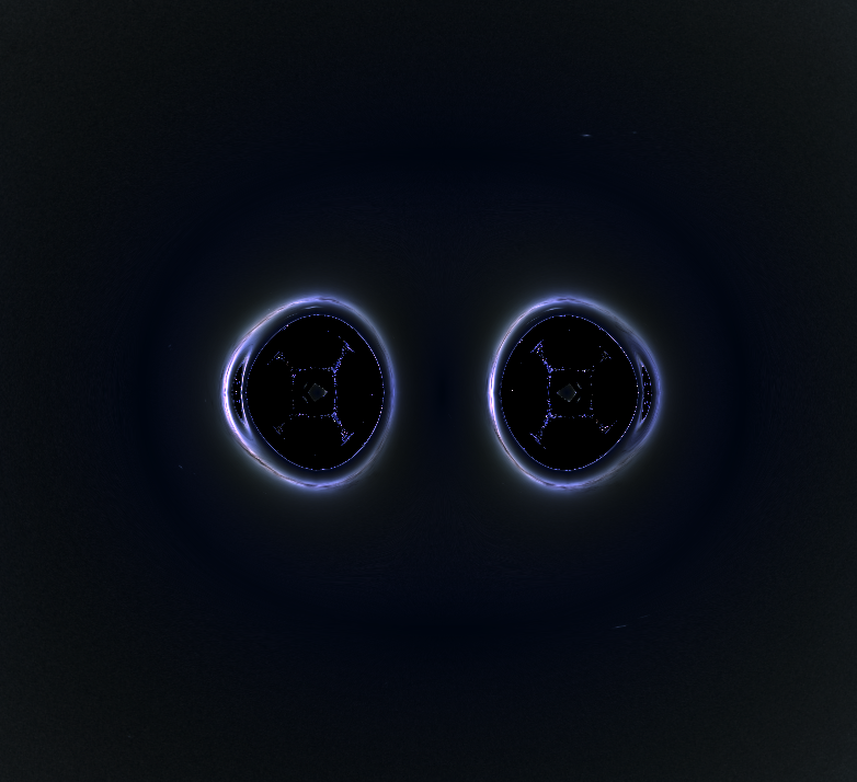
As a final check, we can have a look at the final resting state of the approximate ADM raytracer vs the accurate raytracer, to check how close our results are to each other. They are strictly equivalent in a stationary spacetime, so once the simulation has settled - they should be identical. Given that these are two entirely unrelated techniques, if they match and visually look like black holes - we’re probably close enough with regards to accuracy
Single slice:

All slices:

We can see that the shadow of the black hole is slightly smaller in our full raytracing simulation - likely because of the super low resolution - but they’re very similar. You may also be able to notice that these are clearly both Kerr black holes (as they are asymmetric), and both look to have the same (low) spin value. This is another good sign that we’ve gotten a pretty decent result
Discussion
Overall, I’m extremely happy with the results here. The debugging single-slice raytracing case is incredibly helpful for visualising errors with the black holes as they travel about, and the accurate raytracer has virtually 0 overhead even when unused. It also runs fast-enough that it isn’t too painful to use, which is more than good enough for me
Future improvements
For my use cases, this works well enough. There are a few possible improvements to consider here though
- We can only see a certain amount into the past. We could turn our big buffer chunk into a circular buffer, to exploit this fact and allow for rasterising indefinitely long simulations
- The timestepping could likely be improved
- The time between slices could be dynamic, with more slices when the simulation is changing faster
- Higher order derivatives would let you get better results at a lower resolution. Its likely that swapping to 4th order would be a large improvement, albeit with a reasonable runtime cost
- It would be interesting to explore a version of this where we eliminate $K_{ij}$ and use the ADM geodesic equations. In theory, we only have to take 6 time derivatives for the components of \(\dot{\gamma}_{ij}\), instead of 10 for $\partial_0 g_{\mu\nu}$. This might provide better results, for less computational cost
- Enforcing the null constraint for light rays may improve the quality
Next time
The next article will either be on neutron star collisions (which is a big topic), or gravitational wave extraction. Until then:

Addendum
Why not timelike geodesics?
While the ADM equations of motion presented in this article are applicable to timelike geodesics, in practice integrating them into a simulation is radically different than what you do for lightlike geodesics. Its sufficiently different that - beyond the specific equations themselves - there’s very little commonality in terms of implementation and we’ll need a radically different setup. We’ll be covering timelike geodesics thoroughly when we hit N-body particle dynamics - likely in a few articles time
ADM formalism conversions
| Symbol | Name | Relation to normal GR | Description |
|---|---|---|---|
| $\gamma_{ij}$ | The 3-metric tensor | $g_{ij}$ | Describes curvature on the 3 surface. Symmetric |
| $K_{ij}$ | Extrinsic curvature | $\frac{1}{2 \alpha} (D_i \beta_j + D_j \beta_i - \frac{\partial g_{ij}}{\partial_t})$ | The curvature of the 3 surface with respect to the 4th dimension. Symmetric. Note that $\frac{\partial g_{ij}}{\partial_t} = \frac{\partial \gamma_{ij}}{\partial_t}$ |
| $\alpha$ | Lapse | $\sqrt{-g_{00} + \beta^m \beta_m}$ | Part of the hypersurface normal, which points into the future |
| $\beta^i$ | Shift | $g_{0i}$ | The other part of the hypersurface normal, which points into the future |
BSSN formalism conversions
| Symbol | Name | Relation to ADM | Notes |
|---|---|---|---|
| $W$ | Conformal factor | $det(\gamma_{ij})^{-\frac{1}{6}}$ | Describes the relationship between the ADM variables, and the conformal BSSN variables. $W=0$ at the singularity |
| $\tilde{\gamma}_{ij} $ | Conformal metric tensor | $W^2 \gamma_{ij}$ | Raises and lowers the indices of conformal variables. Inverted as if it were a 3x3 matrix. Symmetric, and has a unit determinant |
| $K$ | Trace of the extrinsic curvature | $\gamma^{ij} K_{ij}$ | |
| $\tilde{A}_{ij}$ | Conformal extrinsic curvature | $W^2 (K_{ij} - \frac{1}{3} \gamma_{ij} K)$ | Trace free, symmetric |
| $\tilde{\Gamma}^i$ | Conformal Christoffel symbol | $\tilde{\gamma}^{jk} \tilde{\Gamma}^i_{jk}$ | Evolved numerically despite having an analytic value from conformal variables, for stability reasons |
| $\alpha$ | Lapse | $\alpha$ | No change |
| $\beta^i$ | Shift | $\beta^i$ | No change |
-
I’m very bad at plugging myself. Contact me at icedshot@gmail.com, or if you’d like - follow my bluesky at @spacejames.bsky.social. I also built a tool for rasterising generic metric tensors, which you might enjoy as well: Raytracer. Please feel free to contact me for any reason, even if you want to just chit chat or nerd out about space. ↩
-
There’s no way to detect if they’ve actually hit a black hole, you have to use a heuristic ↩
-
For timelike geodesics, generally we set $\lambda = \tau$, ie we parameterise our geodesic by proper time ↩
-
In practice the quantity \(E = -p^\mu \mathcal{n}_\mu\) is easier to calculate, as \(\mathcal{n}_\mu = (-\alpha, 0, 0, 0)\), and we already have $p^\mu$ . This means there’s no need to calculate $g_{\mu\nu}$ ↩
-
We could reverse this convention and end up with a similar integrator ↩
-
Its worth noting that due to the cheapness of re-evaluating $dV$ with different values of $V$, you could solve the first equation via fixed point iteration - but due to the relatively weak dependence of the solution on pertubations in $V$, it provides minimal benefits. Particularly, because we’re able to enforce the constraint $V_i V^i = 1$ for lightlike geodesics, we are less exposed to errors in general ↩
-
You can overcommit but it’ll destroy your performance trying to keep that much memory resident simultaneously. Overcommit does play out in our favour though. If you’re thinking that having our giant vram buffer, and our giant bssn state + derivatives allocated all simultaneously will destroy performance, amazingly enough it actually works out perfectly. As far as I can tell, the GPU driver bumps our simulation’s giant history onto the CPU, while the BSSN evolution equations are stored on the GPU. It seems that because we only write to the simulation history while actively simulating (and periodically at that), it simply performs the writes across pcie. This is much better than ending up with a gigantic hitch as 10+ GB of data are streamed onto the GPU. Its a very interesting performance testcase, and it results in virtually 0 overhead in this technique. This allows us to get much higher quality results than if we had to keep all data truly resident ↩
-
If you’re thinking about half precision, its too low quality unfortunately. It results in a simulation that looks like its underwater. If you’re determined to try, consider applying the idea behind (3), ie subtract out the identity matrix from $g_{\mu\nu}$ to improve precision, or use 16-bit fixed point. I haven’t tested either yet and would be interested to know if you do ↩
-
I run these simulations on my desktop pc, and believe me when I say I’d go absolutely bonkers if I couldn’t use it while recording hours of footage for these articles ↩
-
Not a physical acceleration, just a change in our coordinates ↩
-
Interestingly, this pattern might run terribly on datacentre GPUs which don’t have an l3 cache ↩