Numerical Relativity 104: How to build a neutron star - from scratch
Today’s job is very simple, conceptually. We’re going to dig into what it means for something to be a neutron star - how you represent these in general relativity, and all the necessary steps you’ll need to solve along the way to successfully bring one to life in a full numerical relativistic simulation. We’ll be giving them both spin and momentum, because they’re not terribly useful otherwise
This is the first of two articles, with the goal of simulating neutron star collisions:
You should know before we get into this, that we’re stepping into quite an involved process, and there’s a lot of different equations to be solved. No individual step requires any advanced maths or solving techniques - so as long as we try and keep a clear oversight of the overarching process, it’ll be fine
As always, the code is available - for the first half of this article I’ve broken this out into a standalone library here, and the second half of this article is available over here. If you’re looking for someone with a lot of enthusiasm for GPU programming, and who’d rather love to do a PhD in numerical relativity - please give me a shout!1

Background
So, what even is a neutron star anyway?
Fundamentally, a neutron star is a star that is so dense, that it is energetically favourable for the protons and electrons that make it up to combine to form neutrons. As a result, they are made up largely of pure neutrons, under incredible pressure
If this sounds sufficiently exotic that it might pose some fundamental physics problems - then you’d be absolutely correct. Nobody is really super sure exactly what the deal with the physics inside a neutron star is. There’s a few problems:
- You can’t make neutronium in a lab to measure its properties for dozens of very good reasons, not the least of which is because it’d explode very aggressively
- There’s no way to make general relativity and quantum physics get along nicely at these extreme scales. For context, neutron stars have an escape velocity of ~50% the speed of light
- General relativity does not provide a polite solution for a spinning fluid, which means that many of the approximate models that exist are very approximate
- They have the most powerful magnetic fields of anything in the entire universe (allegedly)
This means that a fully predictive approach with a single answer is out of the window, and we’ll have to use some kind of model. The core tool we’ll be using is something called an equation of state (EOS) to encapsulate a neutron star’s physics, which relates various physical parameters together
We won’t be exploring magnetic fields in this article, but you should know they can play an important role in the physics
Bodies in hydrostatic equilibrium
All stars2 (other than black holes) are in hydrostatic equilibrium - this means that their gravity is counterbalanced by an internal pressure. Surprisingly enough, this constraint, along with two other parameters, is enough to fully determine the structure of a star. We also need:
- The density of matter at the centre of the star: $\rho_c$
- An equation of state, which relates the pressure $P$, to the density3 of matter, within the star
So really that’s all a neutron star is for us: Some kind of equation of state, and a central density. With those two pieces, we can use the equations for hydrostatic equilibrium, and end up with a full description of a non spinning body. This gives us:
- The radius $R$ of the star, in Schwarzschild coordinates
- The total (ADM) mass of the star $M$, as well as its rest mass $M_0$4
- The distribution of mass (and pressure, and energy) within the star
In newtonian dynamics (sometimes used as an approximation for GR bodies), the equations governing hydrostatic equilibrium are sufficiently simple that I wouldn’t be writing this article. You’ve probably noticed roughly about now that this article is really very long, so clearly something’s about to go terribly wrong
Overview
This is the game plan for what we’ll be doing:
- First we’ll be constructing a non spinning, isolated neutron star. This will be modelled as a self gravitating fluid in hydrostatic equilibrium. We’ll be solving an equation known as the TOV (Tolman–Oppenheimer–Volkoff) equation, which will fully describe that static star. This is actually a set of partial differential equations, and a good reference for what we’re doing is over here
- Then, we must re-describe that same star as a spinning, moving star. This involves integrating another series of equations, which will be derived from this paper. Its notable that while a real spinning star would be oblate, not modelling this is a deliberate approximation
- Once we have our spinning, moving body, we then have to make it physical by solving for a correction, to make it satisfy our constraints. If you remember the black hole initial conditions, this is the same process. I won’t assume you remember how to do this, but I will assume you can solve a laplacian
- After all of this, we’ll then construct our final hydrodynamic variables - like velocity, density, and energy density. Along the way, we’ll be constructing our ADM variables as well, though this is much simpler
Each of these steps is extremely non trivial, and will be presented in detail. If you’re wondering why we don’t simply directly construct a spinning neutron star through some kind of spinning hydrostatic equilibrium solution, its because the equation simply doesn’t exist. This procedure will work for any number of black holes and neutron stars combined - as long as they don’t overlap - which makes it a very good generalised initial conditions solver
The goal here is to produce the following variables that we can plug into a real hydrodynamic simulation:
| Symbol | Name |
|---|---|
| $\rho_0$ | Rest Mass Density |
| $\epsilon$ | Specific Internal Energy Density |
| $u^\mu$ | Fluid 4-velocity |
| $\gamma_{ij}$ | ADM metric |
| $K_{ij}$ | Extrinsic curvature |
Part 1: Tolman-Oppenheimer-Volkoff (TOV): A non spinning relativistic body in hydrostatic equilibrium
First up: Let’s build a static, non spinning neutron star. What we really want to determine is the distribution of matter within the star, so we can answer the question of its structure. The way that we do this is by calculating the pressure at each point, and then reverse engineering what kind of matter can produce that pressure, via the equation of state
The equation that governs a relativistic, non spinning, spherically symmetric body in hydrostatic equilibrium is called the TOV equation. This is a set of two coupled partial differential equations, which we must solve simultaneously
Wikipedia lists a more complex5 form of the equations, so here’s (6-7) a nicer form (in units of $c=G=1$, Schwarzschild coordinates):
\[\begin{align} \frac{dm}{dr} &= 4 \pi r^2 \mu\\ \frac{dP}{dr} &= -(\mu + P)\frac{m + 4 \pi r^3 P}{r(r-2m)} \end{align}\]Here’s what everything means:
| Symbol | Meaning |
|---|---|
| $r$ | The radius, which parameterises the integration |
| $m$ | The cumulative mass at a radius of less than $r$. Corresponds to the ADM mass |
| $P$ | Pressure at $r$ |
| $\mu$ | Total specific energy density at $r$. This isn’t the energy density integrated, ‘total’ refers to a combination of different energies - but at a specific point |
| $\epsilon$ | Specific internal energy density at $r$ |
| $\rho_0$ | Rest mass density at $r$ (used later) |
This equation is integrated until $P <= 0$. As mentioned previously, we need an equation of state to tie together $\mu$, $\rho_0$ and $P$, which is used implicitly. Here’s how to actually calculate everything, and how it all relates:6
| Symbol | Name | Si Units | Geometric Units | How you should get this variable |
|---|---|---|---|---|
| $r$ | Radius (Schwarzschild coordinates) | $\mathrm{m}$ | $\mathrm{m}$ | Parameterises the integration |
| $m$ | Mass | $\mathrm{kg}$ | $\mathrm{m}$ | Integration variable |
| $P$ | Pressure | $\mathrm{kg}\;\mathrm{m}^{-1} \; \mathrm{s}^{-2}$ | $\mathrm{m}^{-2}$ | Integration variable |
| $\mu$ | Total Specific Energy Density | $\mathrm{kg}\; \mathrm{m}^{-1}\; \mathrm{s}^{-2}$ | $\mathrm{m}^{-2}$ | $\mu = \rho_0 (1 + \epsilon)$ |
| $\epsilon$ | Specific internal energy density | $\mathrm{m}^{2} \; \mathrm{s}^{-2}$ (?)7 | Dimensionless (?) | Equation of state |
| $\rho_0$ | Rest Mass Density | $\mathrm{kg}\; \mathrm{m}^{-3}$ | $\mathrm{m}^{-2}$ | Equation of state |
Here’s some additional equations that are useful:
| Equation | Notes |
|---|---|
| $h = 1 + \epsilon + \frac{P}{\rho_0}$ | Specific enthalpy |
| $\rho_0h = \mu + P$ |
In general, you’ll need to numerically invert the equation of state for some arbitrary equation - which means its time to address equations of state more concretely
Equation of state (EOS)
The simplest equation of state is to model our body as something called a polytrope. This assigns simple relations between our currently unconstrained variables:
- $P = (\Gamma - 1) \rho_0 \epsilon$ - sometimes called the Gamma law equation of state, for a perfect fluid
- $P = K \rho_0^\Gamma$ - the polytropic equation of state
The perfect fluid equation of state is often assumed implicitly. Its worth noting that the polytropic equation of state is actually a subset of the perfect fluid equation of state for an adiabatic process, which means that this is actually only one state model overall. Hydrodynamic simulations often construct stars with a polytropic equation of state, and then evolve them with the perfect fluid equation of state
With this equation of state, I can make you a more useful variable table:
| Symbol | Name | Si Units | Geometric Units | Derivation from $P$ | Derivation from $\rho_0$ |
|---|---|---|---|---|---|
| $P$ | Pressure | $\mathrm{kg}\;\mathrm{m}^{-1} \; \mathrm{s}^{-2}$ | $\mathrm{m}^{-2}$ | $P$ | $K \rho_0^\Gamma$ |
| $\mu$ | Total Energy Density | $\mathrm{kg}\; \mathrm{m}^{-1}\; \mathrm{s}^{-2}$ | $\mathrm{m}^{-2}$ | $(\frac{P}{K})^{1/\Gamma} + \frac{P}{\Gamma-1}$ | $\rho_0 + K \frac{\rho_0^\Gamma}{\Gamma-1}$ |
| $\rho_0$ | Rest Mass Density | $\mathrm{kg}\; \mathrm{m}^{-3}$ | $\mathrm{m}^{-2}$ | $(\frac{P}{K})^{1/\Gamma}$ | $\rho_0$ |
| $K$ | Polytropic Constant (informal) | $\mathrm{kg}^{1-\Gamma} \; \mathrm{m}^{3\Gamma-1}\;\mathrm{s}^{-2}$ 8 | $\mathrm{m}^{2\Gamma-2}$ | ||
| $\Gamma$ | Polytropic index, often $2$ | Dimensionless constant | Dimensionless constant |
This in general is the ‘toy’ equation of state, although it is extremely widely used in these simulations and the literature. A common range for $\Gamma$ is $1.75$ to $2.25$. In this article, while I’ll be going over specific test cases later, you can assume that $\Gamma = 2$ and $K = 123.641$ in units of $c=G=M_\odot=1$
Piecewise equations of state
A more advanced method of modelling a neutron star is to construct a piecewise representation of its equation of state: Essentially, you piece together a bunch of polytropic parts (with different $K$ and $\Gamma$ values) based on some real physics, and ensure some kind of continuity at the boundary between them:
\[\begin{equation} P = \begin{cases} K_0 \rho_0^{\Gamma_0}, & \mathrm{\rho_0 < \rho_0^0} \\ K_1 \rho_0^{\Gamma_1}, & \mathrm{\rho_0^0 < \rho_0 < \rho_0^1} \\ K_n \rho_0^{\Gamma_n}, & \mathrm{\rho_0^{n-1} < \rho_0 < \rho_0^n} \\ \end{cases} \end{equation}\]Using a piecewise perfect fluid equation of state ($P = (\Gamma_i - 1) \rho_0 \epsilon$), we can get the relations for the other variables:
\[\begin{align} \epsilon &= 1 + a_i + \frac{K_i}{\Gamma_i - 1} \rho_0^{\Gamma_i - 1}\\ a_0 &= 0\\ a_i &= a_{i-1} + \frac{K_{i-1}}{\Gamma_{i-1} - 1} (\rho_0^i)^{\Gamma_{i-1} - 1} - \frac{K_i}{\Gamma_i - 1} (\rho_0^i)^{\Gamma_i - 1} \end{align}\]The variable $a_0$ is used to enforce continuity. You’d then calculate $\mu$ from $\epsilon$ and $\rho_0$ as per usual. To find $\rho_0$ you must numerically invert the equation for $P$, which is something we’ll implement later
I’ve converted these equations into our notation, as you should be aware that $\epsilon$ has a different construction in the referenced papers. Note that the $i$ and $n$ in $(p_0^i)$ is an index due to an unfortunate notational clash, and it gets raised to the power of $\Gamma_{i-1} - 1$
Please see here (7) and here (25) for more details
Solving the TOV equations
It’s common to solve these equations in units of $c=G=M_\odot=1$, where $M_\odot$ is the mass of the sun. This is why I’ve provided all the units up above, and we’re going go through converting from SI units, to geometric units ($c=G=1$), to that new unit system ($c=G=M_\odot=1$). In general, you need to redefine mass to avoid the numerics blowing up. The TOV equation itself is agnostic to the dimension of length (which is what is redefined when setting $M_\odot = 1$), so nothing needs to be done there
Unit conversions
The procedure for doing the unit conversion is as follows:
- Given a quantity in SI units $\mathrm{kg}^\alpha \mathrm{m}^\beta \mathrm{s}^\gamma$, convert it to geometric units by dividing by $G^{-\alpha} c^{2 \alpha - \gamma}$. This gives you a new geometrised unit, $\mathrm{m}^{\alpha + \beta + \gamma}$
- Convert the nominal9 mass of the sun, $1.988416 * 10^{30} \mathrm{kg}$, into meters, which is ~$1476.6196 \mathrm{m}$
- Divide your quantity in units of $\mathrm{m}^n$ (eg $\mathrm{m}^2$) by $1476.6196^n$
One thing to note is that $K$ is frequently given in geometric units instead of physical units, so I’ll flag up when the units are wonky. Codewise, this is pretty easy:
///https://www.seas.upenn.edu/~amyers/NaturalUnits.pdf
//https://nssdc.gsfc.nasa.gov/planetary/factsheet/sunfact.html
double geometric_to_msol(double meters, double m_exponent)
{
    double m_to_kg = 1.3466 * pow(10., 27.);
    double msol_kg = 1.988416 * pow(10., 30.);
    double msol_meters = msol_kg / m_to_kg;

    return meters / pow(msol_meters, m_exponent);
}

double msol_to_geometric(double distance, double m_exponent)
{
    return geometric_to_msol(distance, -m_exponent);
}

double si_to_geometric(double quantity, double kg_exponent, double s_exponent)
{
    double G = 6.6743015 * pow(10., -11.);
    double C = 299792458;

    double factor = std::pow(G, -kg_exponent) * std::pow(C, 2 * kg_exponent - s_exponent);

    return quantity / factor;
}

double geometric_to_si(double quantity, double kg_exponent, double s_exponent)
{
    return si_to_geometric(quantity, -kg_exponent, -s_exponent);
}
Initial conditions
Once you’ve got everything in the correct units, we can start solving. Firstly, you might notice that the equations are singular at $r=0$. We’re going to instead start at $r=r_{min}=10^{-6}$
This is the set of initial values to use at $r_{min}$:
| Variable | Value | Notes |
|---|---|---|
| $m$ | $\frac{4}{3} \pi r_{min}^3 \mu_c\;$ | The integral of $\frac{dm}{dr}$, with $\mu_c$ held constant, where $\mu_c$ is $\mu$ at the central density |
| $P$ | $K \rho_c^\Gamma$ | Apply the equation of state to $\rho_c$ (or $\mu_c$ if that’s what you have instead), this is the polytropic specific formula |
| $r$ | $r_{min}$ |
Implementation
Equation of State
For flexibility, I define a very general class of equation of state. This is essentially an adaptor, which automatically generates all the conversions you might want, and you can override specific parts of as necessary
struct base
{
    virtual double mu_to_p0(double mu) const{
        return invert(
        [&](double y){
            return p0_to_mu(y);
        }, mu);
    };

    virtual double p0_to_mu(double p0) const = 0;

    virtual double mu_to_P(double mu) const{return p0_to_P(mu_to_p0(mu));};
    virtual double P_to_mu(double P) const{return p0_to_mu(P_to_p0(P));};

    virtual double P_to_p0(double P) const{
        return invert(
        [&](double y){
            return p0_to_P(y);
        }, P);
    };

    virtual double p0_to_P(double p0) const = 0;

    virtual ~base(){}
};
In theory, we only have to actually define two members here to get everything we’ll need: p0_to_P, and p0_to_mu, and all the rest can be derived via numerical inverts. This isn’t incredible for performance, but depending on your use case, may be either fine or the only option for numerical equations of state
Polytropic equation of state
The functions we need here are simple:
double tov::eos::polytrope::p0_to_mu(double p0) const
{
    double P = p0_to_P(p0);

    return p0 + P / (Gamma - 1);
}

double tov::eos::polytrope::P_to_p0(double P) const
{
    return pow(P/K, 1/Gamma);
}

double tov::eos::polytrope::p0_to_P(double p0) const
{
    return K * pow(p0, Gamma);
}
The implementation of P_to_p0 is useful later when we’re reverse engineering the central density from a specific mass, for performance reasons only
Numerical inversions of the equation of state
Being able to numerically invert a generic function here is going to prove to be quite useful, so lets examine a basic function inverter:
template<typename T>
double invert(T&& func, double y, double lower = 0, double upper = 1, bool should_search = true)
{
    if(should_search)
    {
        //assumes upper > lower
        while(func(upper) < y)
            upper *= 2;
    }

    for(int i=0; i < 10000; i++)
    {
        double lower_mu = func(lower);
        double upper_mu = func(upper);

        double next = 0.5 * lower + 0.5 * upper;

        if(std::fabs(upper - lower) <= 1e-14)
            return next;

        //hit the limits of precision
        if(next == upper || next == lower)
            return next;

        double x = func(next);

        //function assumed to be monotonically increasing
        if(upper_mu >= lower_mu)
        {
            if(x >= y)
                upper = next;
            ///x < y
            else
                lower = next;
        }
        //function assumed to be monotonically decreasing
        else
        {
            if(x >= y)
                lower = next;
            else
                upper = next;
        }
    }

    assert(false);
}
This performs a basic binary search through our function space, until some very low error tolerance is reached. Additionally, for many functions we won’t actually know what our upper bound is, so this guesses it by doubling. That’ll only work for functions which are monotonically increasing, which is true for all our EOS functions
Integration
Its time to integrate the equations. This is done by spotting that these are simple first order in ‘time’ (where $dt=dr$) systems, and can be solved with euler integration10 very straightforwardly. The termination condition is when $P \le 0$, or you can use a small cutoff. I also do a few sanity checks, to make sure we haven’t accidentally constructed a black hole, or something with a suspiciously low mass or radius
Initialising the integration state in units of $c=G=M_\odot=1$ is straightforward:
struct integration_state
{
    double m = 0;
    double p = 0;
};

integration_state make_integration_state(double central_rest_mass_density, double rmin, const eos::base& param)
{
    double mu_c = param.p0_to_mu(central_rest_mass_density);

    double m = (4./3.) * pi * mu_c * std::pow(rmin, 3.);

    integration_state out;
    out.p = param.mu_to_P(mu_c);
    out.m = m;
    return out;
}
Or, if you want to use SI units for the central density:
//p0 in si units
integration_state make_integration_state_si(double central_rest_mass_density, double rmin, const parameters& param)
{
    //kg/m^3 -> m/m^3 -> 1/m^2
    double p0_geom = si_to_geometric(central_rest_mass_density, 1, 0);
    //m^-2 -> msol^-2
    double p0_msol = geometric_to_msol(p0_geom, -2);

    return make_integration_state(p0_msol, rmin, param);
}
The actual integration itself is then easy:
struct integration_dr
{
    double dm = 0;
    double dp = 0;
};

//implements the actual tov equations
std::optional<integration_dr> get_derivs(double r, const tov::integration_state& st, const tov::eos::base& param)
{
    std::optional<integration_dr> out;

    double mu = param.P_to_mu(st.p);

    double p = st.p;
    double m = st.m;

    //black hole + numerical error
    if(r <= 2 * m + 1e-12)
        return out;

    out.emplace();

    out->dm = 4 * pi * mu * std::pow(r, 2.);
    out->dp = -(mu + p) * (m + 4 * pi * r*r*r * p) / (r * (r - 2 * m));
    return out;
}

struct integration_solution
{
    double M_msol = 0;
    double R_msol = 0;

    std::vector<double> rest_density;
    std::vector<double> energy_density;
    std::vector<double> pressure;
    std::vector<double> cumulative_mass;
    std::vector<double> radius; //in schwarzschild coordinates, in units of c=G=mSol = 1
};

///units are c=g=msol=1
std::optional<tov::integration_solution> tov::solve_tov(const integration_state& start,  const tov::eos::base& param, double min_radius, double min_pressure)
{
    integration_state st = start;

    double current_r = min_radius;
    double dr = 1. / 1024.;

    integration_solution sol;

    double last_r = 0;
    double last_m = 0;

    while(1)
    {
        //save current integration state
        sol.rest_density.push_back(param.P_to_p0(st.p));
        sol.energy_density.push_back(param.P_to_mu(st.p));
        sol.pressure.push_back(st.p);
        sol.cumulative_mass.push_back(st.m);
        sol.radius.push_back(current_r);

        last_r = current_r;
        last_m = st.m;

        std::optional<integration_dr> data_opt = get_derivs(current_r, st, param);

        //oops, black hole!
        if(!data_opt.has_value())
            return std::nullopt;

        integration_dr& data = *data_opt;

        //euler integration
        st.m += data.dm * dr;
        st.p += data.dp * dr;
        current_r += dr;

        //something bad happened
        if(!std::isfinite(st.m) || !std::isfinite(st.p))
            return std::nullopt;

        //success!
        if(st.p <= min_pressure)
            break;
    }

    //sanity checks
    if(last_r <= min_radius * 100 || last_m < 0.0001f)
        return std::nullopt;

    sol.R_msol = last_r;
    sol.M_msol = last_m;

    return sol;
}
Testing the implementation
| Case | $\rho_c$ | $K$ | $\Gamma$ | Expected $M$ | Expected $R$ | Notes |
|---|---|---|---|---|---|---|
| C1 (section VII) | $6.235 \times 10^{17}\; \mathrm{kg}\;\mathrm{m}^{-3}$ | $123.641 M_{\odot}^2$ where $c=G=1$11 | $2$ | $1.543 M_\odot$ | $13.4 \; \mathrm{km}$ where $c=G=1$ in Isotropic coordinates | |
| C2 (see after interior) | $1.28 \times 10^{-3} \; \mathrm{m^{-2}}$ where $c=G=M_{\odot} = 1$ | $100$ where $c=G=M_{\odot} = 1$ | $2$ | $1.4 M_{\odot}$ | $14.15\; \mathrm{km}$ where $c=G=1$ in Schwarzschild coordinates | |
| C3 (see: C) | $8.0 \times 10^{-3}$ where $c=G=M_{\odot}=1$ | $100$ where $c=G=M_{\odot} = 1$ | $2$ | $1.447 M_{\odot}$ | unclear | The paper mixes up rest and gravitational mass frequently |
Note that a test case you might find over here uses too low of a value of $N$, and produces incorrect results. Its correct if you bump it up
The code for solving these looks like this:
void case_1()
{
    tov::eos::polytrope param(2, 123.641);
    double paper_p0 = 6.235 * pow(10., 17.);

    double rmin = 1e-6;

    tov::integration_state st = tov::make_integration_state_si(paper_p0, rmin, param);

    tov::integration_solution sol = tov::solve_tov(st, param, rmin, 0).value();

    std::cout << "Solved for " << sol.R_geom() / 1000. << "km" << " Iso " << sol.R_iso_geom() / 1000. << "km " << sol.M_msol << " msols " << std::endl;
}
We’re able to match all these test cases exactly. I get:
C1: Solved for 15.8102km Iso 13.4349km 1.54315 msols
C2: Solved for 14.1461km Iso 11.9894km 1.40021 msols
C3: Solved for 8.60881km Iso 6.29109km 1.44678 msols
Incidentally, the notebook test case I linked gives 14.136399564110704km 1.400270088513766msols when corrected, which is pretty close
We’ll be going over the isotropic <-> Schwarzschild conversion later in this article, just keep in mind that there are two coordinate systems that are commonly used in the literature
Key takeaways from solving TOV
At the end of this process, we’ve gained the ability to fully describe the following variables of our neutron star: rest mass density $\rho_0$, energy density $\mu$, ADM mass $M$, and pressure $P$. I’ve also described how to calculate the rest mass $M_0$ at the end of this article. We’ve now solved the first step in our initial conditions procedure: constructing a spherically symmetric, static neutron star
Next up, we need to give it momentum and spin, which means exiting spherical symmetry - and a new paper to look at
Part 2: Preamble
ADM Refresher
If you can remember how the ADM formalism works, skip this segment. This isn’t really the article for a full redo of the ADM formalism, but here’s a quick overview
The ADM formalism is the process of taking a 4d metric tensor $g_{\mu\nu}$, and splitting it up into a series of 3d slices (called a foliation). Each 3D slice has a number of variables associated with it: $\gamma_{ij},\;K_{ij},\;\alpha,\;\beta^i$. We’ll only be dealing with the ADM formalism, and not the offshoots like BSSN, today. The main things to remember are as follows:
- $\gamma_{ij}$ is the metric on the current 3D slice, and is used to raise and lower indices - eg $M^i = \gamma^{ij} M_i$. $\gamma^{ij}$ is the matrix inverse of $\gamma_{ij}$
- $K_{ij}$ is the extrinsic curvature, and is essentially a momentum term. When it is trace free ($\gamma^{ij}K_{ij} = K = 0$), it is often called $A_{ij}$12
- $\alpha$ and $\beta^i$ are the lapse and shift respectively, and are gauge variables. These are arbitrary and can be picked freely
In a simulation we evolve these slices forwards in time: Here we’re only trying to find the initial variables on a single slice, to plug in somewhere else. This brings the total terms we’re looking to solve for up to these:
| Symbol | Name |
|---|---|
| $\rho_0$ | Rest Mass Density |
| $\epsilon$ | Specific Internal Energy Density |
| $u^\mu$ | Fluid 4-velocity |
| $\gamma_{ij}$ | 3-metric |
| $K_{ij}$ | Extrinsic curvature |
$\beta^i = 0$, and either $\alpha = 1$ or $\alpha$ is calculated from a conformal factor we’ll find later as $\frac{1}{\Phi^2}$
As always, latin indices $ijk$ have the range $[1, 3]$, and greek indices $\mu\nu\kappa$ have the range $[0, 3]$
Numerical integration
We’re about to integrate a lot of equations in 1d, of the form $\int_0^{x_{upper}} f(x) dx$ (where generally, $x$ = $r$). This can be done super duper easily via a routine like this:
///integrates in the half open range [0, index)
auto integrate_to_index = [&](auto&& func, int index)
{
    assert(index >= 0 && index <= samples);

    double last_r = 0;
    std::vector<double> out;
    out.reserve(index);

    double current = 0;

    for(int i=0; i < index; i++)
    {
        //note that this is an isotropic radius coordinate, which we'll get around to shortly
        double r = radius_iso[i];
        double dr = (r - last_r);

        current += func(i) * dr;

        out.push_back(current);

        last_r = r;
    }

    assert(out.size() == index);

    return out;
};
Note that I don’t just return the integral, but the running integral. This means that if we have an integral like this that gets evaluated repeatedly:
\[g(x) = \int_0^{x} f(x) dx\]We can first calculate:
\[\int_0^{x_{upper}} f(x) dx\]And then simply lookup in a table the value of $\int_0^{x} f(x) dx$ for performance reasons. I have everything tabulated in buffers, and always integrate up to indices, which respresent a specific radius $r$
Part 2: Bowen-York Type Initial Data for Binaries with Neutron Stars
The next step we need to do is take our matter distribution - spin it up somehow, and give it some momentum. To do this, we’ll need to transplant it into the ADM formalism, and solve a bunch more equations
The actual paper we’re going to be implementing today is this one. Its going to be a step up in complexity compared to things we’ve solved previously together. One of the key things today is that I’m going to present you with a simpler and fast procedure for implementing this paper, without losing any generality, as I’ve been able to skip some of the complexity. But first, a bit of background:
Fluids in General Relativity
In this paper, our neutron star is modelled as a perfect fluid - this is a very common way to model bodies in general relativity. Matter interactions in GR happen through something called the stress-energy tensor $T_{\mu\nu}$, representing all the matter (and energy) in the spacetime. Components derived from the stress-energy tensor are frequently called ‘sources’ in the literature
The stress-energy tensor for a perfect fluid is calculated as follows:
\[T^{\mu\nu} = (\mu + p) u^\mu u^\nu + p g^{\mu\nu}\]Where $p$ is pressure, $g$ is the metric, and $u^\mu$ is the fluid’s 4-velocity. $\mu$ is still the total specific energy density. These components are then projected onto our hypersurface (ie, we’re sticking this into the ADM formalism). Here, this paper actually only requires two parts of that projection, which are defined as follows13:
\[\begin{align} \mu_H &= n^\mu n^\nu T_{\mu\nu}\\ S^i &= -\gamma^{i\mu}n^\nu T_{\mu\nu} \end{align}\]Where $n^\mu$ is the hypersurface normal. In fluid terms:
\[\begin{align} \mu_H &= (\mu + p)W^2 - p \\ S^i &= (\mu + p) W u^i\\ \end{align}\]$W$ is a Lorentz factor ($=-n_\mu u^\mu$), and $u^i$ is the spatial components of the fluid’s 4-velocity. These two variables fully encompass our fluid’s state here, and also fully determine the structure of our spacetime. Calculating these is a major goal here
$S^i$ will be broken up into two parts: An angular momentum part, and a linear momentum part. These are used implicitly to calculate the extrinsic curvature
Starting off
For consistency14, we’ll be keeping our existing notation, and below is the conversions we’ll make:
| Symbol | This article | Paper |
|---|---|---|
| Total energy density | $\mu$ | $\rho$ |
| Pressure | $P$ or $p$ | $p$ |
The swap from $P$ to $p$ is because $P^i$ will be used for the ADM momentum
The basic idea for many kinds of initial conditions is based on the principle of a conformal transform, where your variables are multiplied by a conformal factor: $\Phi$. In this paper, our variables are transformed as follows:
\[\begin{align} \gamma_{ij} &= \Phi^4 \bar{\gamma}_{ij}\\ A_{ij} &= \Phi^{-2} \bar{A}_{ij}\\ \mu_H &= \Phi^{-8} \bar{\mu}_H\\ S^i &= \Phi^{-10} \bar{S}^i \end{align}\]Here’s what everything is:
| Variable | Meaning | Primary solution method | Notes |
|---|---|---|---|
| $\Phi$ | Conformal factor | Laplacian, via the hamiltonian constraint | |
| \(\bar{\gamma}_{ij}\) | Conformal metric tensor | We’ve already got it | Conformal flatness is imposed, ie we make it the identity matrix |
| $\bar{A}_{ij}$ | Conformal extrinsic curvature | Derived from our physical parameters (mass, momentum, spin), requires some numerical integration | Trace-free’dom is imposed, which is called maximal slicing ($K=0$) |
| $\bar{\mu}_H$ | The ADM projection of part of the stress-energy tensor, conformally transformed | Derived from our TOV solution, requires some numerical integration | |
| $\bar{S}^i$ | The ADM projection of part of the stress-energy tensor, conformally transformed | Calculated via a similar process to $\bar{A}_{ij}$, requires some numerical integration (surprise!) |
Anything with a bar over it is a conformal variable, and their indices are raised and lowered with the conformal metric. This is the same conformal decomposition as the black hole initial conditions we’ve discussed previously15
Conformal flatness + maximal slicing gives us a familiar looking constraint to solve (18):
\[\partial^i \partial_i \Phi = -\frac{1}{8} \Phi^{-7} \bar{A}_{ij} \bar{A}^{ij} - 2 \pi \Phi^{-3} \bar{\mu}_H\]Solving this equation - and calculating $\bar{A}^{ij}$, $\bar{\mu}_H$, and $\bar{S}^i$ - is most of the work of what we’ll be doing. One thing to note is that any time you see a $\pi$, its a sure fire bet that it means there are matter terms involved. The final hydrodynamic variables will be recovered after we’ve solved the above
This paper in theory lets us solve the TOV equations in a conformally flat spacetime, via (77-79), but I’ve deliberately skipped this step, as solving the TOV equations directly is much simpler. In general I wouldn’t recommend implementing section VI (other than (83-84)), and I think (82) is incorrect unfortunately
Implementing this paper
The procedure we’ll be using is as follows:
- Solve for $\Phi_{tov}$, a conformal factor for the isotropic TOV solution, to make it conformally flat
- Construct conformal hydrodynamic variables from our TOV hydrodynamic variables
- Use these, as well as the linear momentum and angular momentum to calculate $\bar{A}_{ij}$
- Use that $\bar{A}_{ij}$ solution to construct $\Phi$, the real conformal factor
- Construct the final real hydrodynamic variables from the conformal ones defined earlier
- Calculate the final ADM quantities
- Go outside and celebrate with our loved ones who miss us
Solving for $\Phi_{tov}$
First off, we need to start over in section VI. Given that we a-priori have our matter distribution, we don’t need to solve for $\alpha$, or $\Theta$ luckily, and the only variable we need is $\Phi_{tov}$. There’s a nicer way of solving for $\Phi_{tov}$ than specified in the paper, but first we should talk about $\bar{r}$. One thing that absolutely must be noted is that the paper we’re working on is in isotropic coordinates with the radial coordinate $\bar{r}$. Up until now, we’ve been working in Schwarzschild coordinates with the radial coordinate $r$. We’re going to have to perform a conversion between the two: the conversion function is defined as follows (24 + 25):
\[\begin{align} \bar{r} &= C\;r\;\mathrm{exp}(\int^r_0 \frac{1 - (1 - 2 \frac{m}{r})^{\frac{1}{2}}}{r(1 - 2\frac{m}{r})^{\frac{1}{2}}} dr)\\ C &= \frac{1}{2R}(\sqrt{R^2 - 2MR} + R - M)\; \mathrm{exp}(-\int^R_0 \frac{1 - (1 - 2 \frac{m}{r})^{\frac{1}{2}}}{r(1 - 2\frac{m}{r})^{\frac{1}{2}}} dr) \end{align}\]Where $R$ is the radius of the star in Schwarzschild coordinates, and $M$ is the total ADM mass (ie the final value of $m$ after solving TOV. $m(r)$ is still cumulative mass). $C$ is a constant. Technical details of how this works is available on the linked page16, and its a good read if you’re interested in how we get here
Integrating this (code link) is moderately straightforward, and can be done by keeping a running summation of the integral within $\mathrm{exp}$:
std::vector<double> initial::calculate_isotropic_r(const tov::integration_solution& sol)
{
    std::vector<double> r_hat;
    double last_r = 0;
    double log_rhat_r = 0;

    for(int i=0; i < (int)sol.radius.size(); i++)
    {
        double r = sol.radius[i];
        double m = sol.cumulative_mass[i];

        //note that we're integrating with respect to the schwarschild radial coordinate
        double dr = r - last_r;

        double rhs = (1 - sqrt(1 - 2 * m/r)) / (r * sqrt(1 - 2 * m/r));

        log_rhat_r += dr * rhs;

        double lr_hat = exp(log_rhat_r);

        r_hat.push_back(lr_hat);

        last_r = r;
    }

    {
        double final_r = r_hat.back();

        double R = sol.radius.back();
        double M = sol.cumulative_mass.back();

        double scale = (1/(2*R)) * (sqrt(R*R - 2 * M * R) + R - M) / final_r;

        for(int i=0; i < (int)sol.radius.size(); i++)
        {
            r_hat[i] *= sol.radius[i] * scale;
        }
    }

    return r_hat;
}
To get back to the topic at hand, note that we’re looking for a $\Phi_{tov}$ for a metric defined as follows (73):
\[ds^2 = -\alpha^2(\bar{r}) dt^2 + (\Phi_{tov}(\bar{r}))^4(d\bar{r}^2 + \bar{r}^2 d\Omega)\]The einstein toolkit page lists TOV in isotropic coordinates as:
\[ds^2 = -e^{2\phi} dt^2 +e^{2\Lambda}(d\bar{r}^2 + \bar{r}^2 d\Omega^2)\]We can see that $e^{2\Lambda} = \Phi_{tov}^4$. And, helpfully, someone smarter17 than I am has worked out that $e^{\Lambda} = \frac{r}{\bar{r}}$
std::vector<double> initial::calculate_tov_phi(const tov::integration_solution& sol)
{
    auto isotropic_r = calculate_isotropic_r(sol);
    int samples = sol.radius.size();

    std::vector<double> phi;
    phi.resize(samples);

    for(int i=0; i < (int)sol.radius.size(); i++)
    {
        phi[i] = pow(sol.radius[i] / isotropic_r[i], 1./2.);
    }

    return phi;
}
This is a much nicer way of calculating this quantity, as $\Phi_{tov} = (\frac{r}{\bar{r}})^\frac{1}{2}$. Do note as an implementation detail, when you’re looking up eg a pressure at a radius, you’ll want to ensure that you have the ability to look it up by isotropic radius. Ie we need to keep on hand the function $r = f(\bar{r})$, which you should tabulate somewhere
From now on, our $r$ coordinate is always isotropic. Variables such as $\bar{\mu}$ should be considered a function of isotropic radius. In general, if you’re operating similarly to how I am where your variables are stored in buffers and indexed instead of actually looking things up by the radius, you don’t need to do anything
Calculating the conformal hydrodynamic variables
Once we have $\Phi_{tov}$, this is straightforward. The new conformal variables are defined as such (83-84), keeping in mind that we’re using slightly different notation from the paper:
\[\begin{align} \bar{\mu} &= \Phi_{tov}^8 \mu_{tov}\\ \bar{p} &= \Phi_{tov}^8 p_{tov} \end{align}\]These are the only two variables you now need from the TOV solution. You’ll also need the equation of state for later, so keep it around somewhere
Calculating $\bar{A}^{ij}$
The code for this section is available over here
From here, its time to dig into the really fun bits - this is the main chunk of the paper. As with our black hole solution, we have two parameters we can specify: the ADM momentum $P^i$, and the ADM angular momentum $J^i$18. The contribution from each of these to the extrinsic curvature is broken up into two equations: (51), and (54) - which we simply sum together
$P^i$ (linear momentum)
To calculate the contribution from the linear momentum, we have this equation:
\[\begin{align} \bar{A}^{ij}_P &=\frac{3Q}{2r^2}(P^i l^j + P^j l^i - (\eta^{ij} - l^i l^j)(P^k l_k)) \\ &+ \frac{3C}{r^4} (P^i l^j + P^j l^i + (\eta^{ij} - 5l^i l^j)(P^k l_k))\\ \end{align}\]Here’s what everything means
| Symbol | Definition |
|---|---|
| $P^i$ | ADM linear momentum |
| $r$ | Coordinate distance (in isotropic coordinates) from the neutron star’s origin |
| $\eta^{ij}$ | The inverse of the conformally flat metric tensor (here: the identity matrix) |
| $l^i$ | $l^i=\frac{x^i}{r}$, a unit radial vector |
| $Q$ and $C$ | We’ll get to these |
The quantities here are trivial to calculate, except for $Q$ and $C$. This is where the information in this paper gets a bit.. scattered, so I’m simply going to present the order of things to calculate
$\mathcal{M}$ | Constant
The first thing we need is to calculate $\mathcal{M}$. This is straightforward via (59)
\[\mathcal{M} = 4\pi \int^{r_0}_0 (\bar{\mu} + \bar{p}) r^2 dr\]Integrating this is a straightforward piecewise numerical integration. $r_0$ is the isotropic radius of our neutron star, and $r$ is the integration variable. Note that this quantity is not the same as $M$
I won’t make you read the code for every single one of these variables, but here’s an example for $\mathcal{M}$:
    double M = 4 * M_PI * integrate_to_index([&](int idx)
    {
        double r = radius_iso[idx];

        return (mu_cfl[idx] + pressure_cfl[idx]) * pow(r, 2.);
    }, samples).back();
This integrates over every sample
$\sigma$ | Function of radius
Next up, we’ll calculate sigma. This is done via (57):
\[\sigma = \frac{\bar{\mu} + \bar{p}}{\mathcal{M}}\]$Q$ and $C$ | Functions of radius
These are specified as follows:
\[\begin{align} Q(r) &= 4 \pi \int^r_0 \sigma x^2\; dx\\ C(r) &= \frac{2}{3} \pi \int^r_0 \sigma x^4\; dx\\ \end{align}\]When $r > r_0$, $Q(r)=1$, and you should enforce this. The paper does not specify a value for $C(r)$ where $r > r_0$, so I set $C(r) = C(r_0)$ in this region
I personally found the $r’$ notation to be somewhat unintuitive when I first read this paper19, given that its also used for differentiation, so I’ve swapped the notation to make it clearer that it is an integration variable. Note that $\sigma$ is also a function, so here we’d be doing $\sigma(x)$
Here’s what implementing $Q$ looks like:
    std::vector<double> Q = integrate_to_index([&](int idx)
    {
        double r = radius_iso[idx];

        return 4 * M_PI * sigma[idx] * r*r;
    }, samples);
All the other variables are functionally identical in implementation. I’ll get around to the implementation of $\bar{A}^{ij}_P$ soon
$J^i$ (angular momentum)
The equation for this is (54):
\[\bar{A}^{ij}_J =\frac{6}{r^3}l^{ (i } \epsilon^{j)kl} J_k l_l N\]Here’s what everything means
| Symbol | Definition |
|---|---|
| $J^i$ | ADM angular momentum (lower with $\eta_{ij}$, here the identity matrix) |
| $r$ | Coordinate distance (in isotropic coordinates) from the neutron stars origin |
| $l^i$ | $l^i=\frac{x^i}{r}$, a unit radial vector (lower with $\eta_{ij}$) |
| $N$ | We’ll get to this |
| $\epsilon^{ijk}$ | The levi civita symbol (with its indices raised) |
As previously, we’ll dig into the procedure for calculating $N$, and linearise the procedure because the functions are a bit scattered
$\mathcal{N}$ | Constant
You might be wondering if having two variables named $\mathcal{N}$ and $N$ might have resulted in days of confusion for a poor lost developer several years ago, who was reading this as an early paper in their NR journey when they didn’t know any better than to be hypervigilant of notational issues, or even that calligraphic styles could be functional
Anyway. Implementing this is under (64):
\[\mathcal{N} = \frac{8 \pi}{3} \int^{r_0}_0 (\bar{\mu} + \bar{p}) r^4\; dr\]Where $r_0$ is the isotropic radius of our neutron star, and $r$ is the integration variable. Perhaps this goes without saying for people with better reading skills, but this function is not $N$
$\kappa$ | Function of radius
(62)
\[\kappa =\frac{\bar{\mu} + \bar{p}}{\mathcal{N}}\]When $r > r_0$, $\kappa(r) = 0$
$N$ | Function of radius
(55)
\[N(r) = \frac{8 \pi}{3} \int^r_0 \kappa x^4\;dx\]Remembering that $\kappa(x)$ is a function, and $x$ is the integration variable
When $r>r_0$, $N(r) = 1$. You should enforce this
This is when I swap to cartesian coordinates
Up until now, we’ve been solving everything in one dimension as a function of radius - TOV is spherically symmetric, so it works great. Unfortunately, the extrinsic curvature has no obligation to be a simple function of radius. That means that I pick the boundary between the radial functions calculated above, and the extrinsic curvature calculations, to be where I discretise to 3D and port everything to the GPU
I pass all the constituent components that I need to calculate $\bar{A}^{ij}_P$ and $\bar{A}^{ij}_J$ to the GPU in many buffers and calculate it in 3D directly. Here’s the basic form of what I’m doing on the host for buffers, which includes a double -> float conversion given that GPUs are a bit allergic to double precision
    auto to_gpu = [&](const std::vector<double>& in)
    {
        std::vector<float> f;
        f.reserve(in.size());

        for(auto& i : in)
            f.push_back(i);

        cl::buffer buf(ctx);
        buf.alloc(sizeof(cl_float) * in.size());
        buf.write(cqueue, f);
        return buf;
    };

    cl::buffer cl_Q = to_gpu(Q);
    cl::buffer cl_C = to_gpu(C);
    cl::buffer cl_uN = to_gpu(unsquiggly_N);

    cl::buffer cl_sigma = to_gpu(sigma);
    cl::buffer cl_kappa = to_gpu(kappa);

    cl::buffer cl_mu_cfl = to_gpu(mu_cfl);
    cl::buffer cl_pressure_cfl = to_gpu(pressure_cfl);
    cl::buffer cl_radius = to_gpu(radius_iso);
Implementing the extrinsic curvature on the GPU is only mildly horrendous. First up, we need the ability to interpolate buffers by their isotropic radius, which includes a boundary condition for the exterior of the star
auto get = [&](single_source::buffer<valuef> quantity, valuef upper_boundary, valuef r)
{
    mut<valuef> out = declare_mut_e(valuef(-1.f));
    mut<valuei> found = declare_mut_e(valuei(0));

    //below our minimum radius sample
    if_e(r <= radius_b[0], [&]{
        //implicitly uses quantity[0] as lower bound
        as_ref(out) = quantity[0];
        as_ref(found) = valuei(1);
    });

    //exterior to the neutron star
    if_e(r > radius_b[samples - 1], [&]{
        //use explicitly passed in upper bound
        as_ref(out) = upper_boundary;
        as_ref(found) = valuei(1);
    });

    //lies within the neutron star samples we have
    if_e(r > radius_b[0] && r <= radius_b[samples - 1], [&]{
        mut<valuei> index = declare_mut_e(valuei(0));

        //for every sample
        for_e(index < samples - 1, assign_b(index, index+1), [&]{
            valuef r1 = radius_b[index];
            valuef r2 = radius_b[index + 1];

            //found the radial coordinate we passed in
            if_e(r > r1 && r <= r2, [&]{
                valuef frac = (r - r1) / (r2 - r1);

                //linearly interpolate our quantity based on the radius
                as_ref(out) = mix(quantity[index], quantity[index + 1], frac);
                as_ref(found) = valuei(1);

                break_e();
            });
        });
    });

    if_e(found == 0, [&]{
        print("Borked get\n");
    });

    return declare_e(out);
};
I bet you haven’t missed the weird GPU language I’m using20. Linear interpolation is used here, but in general the TOV solution contains a huge number of samples compared to the grid resolution (which is $199^3$ for no particular reason), so its a non problem - you can easily get away with nearest-neighbour
Next comes the actual implementation of the extrinsic curvature
//function of grid position
auto get_AIJ = [&](v3f fpos)
{
    v3f body_pos = lbody_pos.get();
    v3f world_pos = grid_to_world(fpos, dim, scale);

    v3f from_body = world_pos - body_pos;

    valuef r = from_body.length();
    pin(r);

    v3f li = from_body / max(r, valuef(0.000001f));

    //look up functions by isotropic radius
    valuef Q = get(Q_b, 1.f, r);
    valuef C = get(C_b, C_b[samples-1], r);
    valuef N = get(uN_b, 1.f, r);

    v3f li_lower = flat.lower(li);
    v3f P = linear_momentum.get();
    v3f J = angular_momentum.get();

    valuef pk_lk = dot(P, li_lower);

    tensor<valuef, 3, 3> AIJ_p;

    valuef cr = max(r, valuef(0.00001f));

    //calculate linear part
    for(int i=0; i < 3; i++)
    {
        for(int j=0; j < 3; j++)
        {
            AIJ_p[i, j] = (3 * Q / (2 * cr*cr)) *   (P[i] * li[j] + P[j] * li[i] - (iflat[i, j] - li[i] * li[j]) * pk_lk)
                         +(3 * C / (cr*cr*cr*cr)) * (P[i] * li[j] + P[j] * li[i] + (iflat[i, j] - 5 * li[i] * li[j]) * pk_lk);
        }
    }

    auto eijk = get_eijk();

    //super unnecessary, being pedantic
    auto eIJK = iflat.raise(iflat.raise(iflat.raise(eijk, 0), 1), 2);

    tensor<valuef, 3, 3> AIJ_j;

    v3f J_lower = flat.lower(J);

    //calculate angular part
    for(int i=0; i < 3; i++)
    {
        for(int j=0; j < 3; j++)
        {
            valuef sum = 0;

            for(int k=0; k < 3; k++)
            {
                for(int l=0; l < 3; l++)
                {
                    sum += (3 / (cr*cr*cr)) * (li[i] * eIJK[j, k, l] + li[j] * eIJK[i, k, l]) * J_lower[k] * li_lower[l] * N;
                }
            }

            AIJ_j[i, j] += sum;
        }
    }

    return AIJ_p + AIJ_j;
};
Calculating $\Phi$, the conformal factor
For every star, we now have $\bar{\mu}$, $\bar{p}$, and $\bar{A}^{ij} = \bar{A}^{ij}_P + \bar{A}^{ij}_J$. We’ll need to combine the individual per-star pieces together, and then solve the final part of our puzzle (22):
\[\Delta \Phi = -\frac{1}{8} \Phi^{-7} \bar{A}_{ij} \bar{A}^{ij} - 2 \pi \Phi^{-3} \bar{\mu}_H\]This is a standard laplacian, and what we’ll be using to solve for the conformal factor. We’re going to go over the details of how to perform our full construction after we finish up our next step, which is solving for $\bar{\mu}_H$. Whatever it is, it can’t be that bad, right?

Solving for $\bar{\mu}_H$
The definition can be found by applying $\Phi_{tov}^8$ to $\mu_H$ (6 + 20):
\[\bar{\mu}_H = (\bar{\mu} + \bar{p})W^2 - \bar{p}\]Which will be set to $0$ when $r>r_0$. What’s $W$?
$W$, aka the Lorentz factor
I’ve moved an extremely extended discussion about the correct way to calculate this variable to the end of the article for flow reasons. If you’re ever interested in the behind-the-scenes development of these articles, you can skip over there to enjoy my frustration, as well as some maths. This deviates from the procedure specified in the paper, as it does not work in our case
To cut a long story short, we’ll need to plug some source $\bar{S}^i$ into the following equation to calculate the Lorentz factor (27):
\[W^2 = \frac{1}{2}\left [1 + \sqrt{1 + \frac{4 \bar{\gamma}_{ij} \bar{S}^i \bar{S}^j}{(\bar{\mu} + \bar{p})^2}}\right]\\\]There are two ways to calculate $\bar{S}^i$:
Way the first
For this method, we have to calculate two individual sources - a linear part $\bar{S}^i_P$ (32), and an angular part $\bar{S}^i_J$ (33), then sum them together:
\[\begin{align} \bar{S}^i_P &= P^i \sigma \\ \bar{S}_i^J &= \epsilon_{ijk} J^j x^k \kappa \\ \bar{S}^i_{summed} &= \bar{S}^i_P + \bar{\gamma}^{ij}\bar{S}_j^J \end{align}\]where $\epsilon_{ijk}$ is the levi civita symbol, and $x^k$ is the world position relative to the centre of the neutron star
auto Si_direct_sum = [&]()
{
    v3f P = linear_momentum.get();
    v3f J = angular_momentum.get();

    valuef sigma = get(sigma_b, 0.f, r);
    valuef kappa = get(kappa_b, 0.f, r);

    auto eijk = get_eijk();

    v3f Si_P = P * sigma;
    v3f S_iJ;

    for(int i=0; i < 3; i++)
    {
        for(int j=0; j < 3; j++)
        {
            for(int k=0; k < 3; k++)
            {
                S_iJ[i] += eijk[i, j, k] * J[j] * from_body[k] * kappa;
            }
        }
    }

    v3f tSi = Si_P + iflat.raise(S_iJ);
    pin(tSi);
    return tSi;
};
Way the second
The momentum constraint can be used to calculate a source from the extrinsic curvature for a single star:
\[\bar{\nabla}_j \bar{A}^{ij} = 8 \pi \bar{S}^i\]Remember that the conformal metric tensor is flat, so $\bar{\nabla}_j \bar{A}^{ij} = \partial_j \bar{A}^{ij}$. Here, $\bar{A}^{ij}$ is the two summed components of the extrinsic curvature for a single star only: $\bar{A}^{ij} = \bar{A}^{ij}_P + \bar{A}^{ij}_J$, and this is not the total extrinsic curvature for all stars. You don’t need to worry about imposing a boundary condition exterior to the star, as $W^2$ is multiplied by matter terms
auto Si_from_AIJ = [&]()
{
    tensor<valuef, 3> Si;

    for(int i=0; i < 3; i++)
    {
        valuef sum = 0;

        for(int j=0; j < 3; j++)
        {
            float off = 0.01;

            v3f offset;
            offset[j] = off;

            v3f fpos = (v3f)pos;

            tensor<valuef, 3, 3> right = get_AIJ(fpos + offset);
            tensor<valuef, 3, 3> left = get_AIJ(fpos - offset);
            pin(right);
            pin(left);

            auto diff = (right - left) / (off * 2 * scale);

            sum += diff[i, j] / (8 * M_PI);
            pin(sum);
        }

        Si[i] = sum;
    }

    return declare_e(Si);
};
These produce identical results - way the first is slightly better, and is what is turned on by default. Once we’re here, $\bar{\mu}_H$ is easy to calculate
    valuef mu_cfl = get(mu_cfl_b, 0.f, r);
    valuef pressure_cfl = get(pressure_cfl_b, 0.f, r);

    v3f Wu_hi = Si / max(mu_cfl + pressure_cfl, valuef(1e-12f));

    valuef W2 = 0.5f * (1 + sqrt(1 + 4 * flat.dot(Wu_hi, Wu_hi)));

    valuef mu_h = (mu_cfl + pressure_cfl) * W2 - pressure_cfl;
Solving the laplacian, finally
Here, I’m going to describe how to mix together neutron stars, and black holes. For both neutron stars, and black holes, we have an extrinsic curvature $\bar{A}^{ij}$. For black holes, use the procedure as specified here in a previous article to get their extrinsic curvature. This is great, we simply sum every extrinsic curvature linearly, and then calculate $\bar{A}^{ij} \bar{A}_{ij}$ for all objects
Next up, we need to do a bit of work. First off, we need to remember that we can express our conformal factor as $\Phi = 1 + u + F$. $u$ is a correction, and what we solve for in the laplacian. We didn’t dig into this, but as black holes have no matter distribution, the term $F$ (originally called: $\frac{1}{a}$) is to stop the solution from being trivially flat. This isn’t a problem for neutron stars, as you can see in our laplacian we have the term:
\[- 2 \pi \Phi^{-3} \bar{\mu}_H\]Which is a matter term on the right hand side, and prevents it from being trivially flat. To make this all interoperate correctly and give correct solutions, I’ll lay out how this works:
| Type | Function |
|---|---|
| Neutron Star | $F_{(i)} = 0$ |
| Black Hole | $F_{(i)} = \frac{m_i}{2 \mid \overrightarrow{r} - \overrightarrow{x}_{(i)} \mid}$ |
To calculate $F$, sum over $F_{(i)}$ for every object
The last thing to do is figure out what to do with our individual $\bar{\mu}_H$ terms. Luckily, you simply sum these21. To make this super explicit:
\[\begin{align} \bar{A}_{ij}^{sum} &= \sum^N_{k=1} \bar{A}_{ij}^{(k)}\\ F^{sum} &= \sum^N_{k=1} F_{(k)} \\ \bar{\mu}^{sum}_H &= \sum^N_{k=1} \bar{\mu}_H^{(k)}\\ \Phi &= 1 + u + F^{sum}\\ \Delta u &= -\frac{1}{8} \Phi^{-7} \bar{A}_{ij}^{sum} \bar{A}^{ij}_{sum} - 2 \pi \Phi^{-3} \bar{\mu}^{sum}_H \end{align}\]That’s it, we’re good to go. From here on, its just a standard laplacian of exactly the same form we solved previously, with nothing special going on
This allows you to now calculate these non conformal variables:
| Name | Symbol | Value |
|---|---|---|
| Metric Tensor | \(\gamma_{ij}\) | \(\Phi^4 \bar{\gamma}_{ij}\) |
| Extrinsic Curvature | \(K_{ij}\) | \(\Phi^{-2} \bar{A}_{ij}\) |
| Initial Adm Matter Source | \(\mu_H\) | \(\Phi^{-8} \bar{\mu}_H\) |
| Initial Adm Matter Source | \(S^i\) | \(\Phi^{-10} \tilde{S}^i\) |
Note that two of these - the metric, and extrinsic curvature, are two of the initial variables we were trying to solve for. We still need to do a bit of work for the hydrodynamics

Recovering the hydrodynamic variables
The code for this section is available over here, see init_hydro
The variables $S^i$ and $\mu_H$ are not actually hydrodynamic quantities - but instead projections of the stress-energy tensor - and so we have to construct our final real quantities that we could plug into a fluid dynamics simulation
| Symbol | Name |
|---|---|
| $W$ aka $u^0$ | The Lorentz factor |
| $u^i$ | Fluid 4-velocity (the spatial components) |
| $\rho_0$ | Rest mass density |
| $\mu$ | Total mass-energy density |
| $p$ | Pressure |
We unfortunately cannot simply transform our conformal variables from earlier. There are two issues:
- They no longer match up to each other - an equation of state is generally non linear, so our variables wouldn’t correspond correctly after a conformal transform
- They are no longer physically relevant. $\mu_H$ is physical because we’ve solved for a conformal factor that makes it satisfy our constraints exactly, and $S^i$ fulfills our momentum constraint. Using the old conformal variables wouldn’t generate a solution that satisfies the physical constraints
We must construct our hydrodynamic variables from $S^i$ and $\mu_H$ only. To do this, we have the following equations (69-71):
\[\begin{align} \mu_H &= (\mu + p) W^2 - p \\ \gamma_{ij} S^i S^j &= (\mu + p)^2 W^2 (W^2 - 1) \end{align}\]Initially this might seem a tad unsolvable, but we have an equation of state that you can use to tie together $\mu$ and $p$. This paper omits the way you should solve these equations (which is non trivial), and so I’ll detail a procedure I came up with for solving this. You’ll also need the ability to go from $\mu$ -> $p$, ie $p = f(\mu)$
- Make an initial guess for $W_0=1$ and $\mu_0 = \mu_H$
- Calculate $W_{n+1} = \frac{\sqrt{1 + \sqrt{4 \frac{\gamma_{ij} S^i S^j}{(\mu_n + p)^2} + 1}}}{\sqrt{2}}$ (from eq 2., equivalent to (27))
- Numerically find a $\mu$ such that $(\mu_n + p) W_{n+1}^2 - p = \mu_H$, giving $\mu_{n+1}$. I do a simple linear search
- Iterate until the desired accuracy is reached
This is applying fixed point iteration to these two equations to solve them simultaneously. Once you’ve solved for $W$ and $\mu$, then calculate $u^i = \frac{S^i}{(\mu + p)W}$. The full fluid 4-velocity is $(W, u^i)$
Implementing this isn’t super fun:
    valuef max_density = eos_data.max_densities[index];
    valuef max_mu = eos_data.max_mus[index];

    bssn_args args(pos, dim, in);

    //performs a linear scan to invert P -> p0
    auto pressure_to_p0 = [&](valuef P)
    {
        valuei offset = index * eos_data.stride.get();

        mut<valuei> i = declare_mut_e(valuei(0));
        mut<valuef> out = declare_mut_e(valuef(0));

        for_e(i < eos_data.stride.get() - 1, assign_b(i, i+1), [&]{
            valuef p1 = eos_data.pressures[offset + i];
            valuef p2 = eos_data.pressures[offset + i + 1];

            if_e(P >= p1 && P <= p2, [&]{
                valuef val = (P - p1) / (p2 - p1);

                as_ref(out) = (((valuef)i + val) / (valuef)eos_data.stride.get()) * max_density;

                break_e();
            });
        });

        if_e(i == eos_data.stride.get(), [&]{
            print("Error, overflowed pressure data\n");
        });

        return declare_e(out);
    };

    //tabulated p0 -> P
    auto p0_to_pressure = [&](valuef p0)
    {
        valuei offset = index * eos_data.stride.get();

        valuef idx = clamp((p0 / max_density) * (valuef)eos_data.stride.get(), valuef(0), (valuef)eos_data.stride.get() - 2);

        valuei fidx = (valuei)idx;

        return mix(eos_data.pressures[offset + fidx], eos_data.pressures[offset + fidx + 1], idx - floor(idx));
    };

    valuef mu_h_cfl = mu_h_cfl_b[pos, dim];
    valuef phi = cfl_b[pos, dim] + u_correction_b[pos, dim];
    //with raised index
    v3f Si_cfl = {Si_cfl_b[0][pos, dim], Si_cfl_b[1][pos, dim], Si_cfl_b[2][pos, dim]};

    valuef mu_h = mu_h_cfl * pow(phi, -8);
    //with raised index
    v3f Si = Si_cfl * pow(phi, -10);

    valuef Gamma = get_Gamma();

    //tabulated mu -> p0
    auto mu_to_p0 = [&](valuef mu)
    {
        valuei offset = index * eos_data.stride.get();

        valuef idx = clamp((mu / max_mu) * (valuef)eos_data.stride.get(), valuef(0), (valuef)eos_data.stride.get() - 2);

        valuei fidx = (valuei)idx;

        return mix(eos_data.mu_to_p0[offset + fidx], eos_data.mu_to_p0[offset + fidx + 1], idx - floor(idx));
    };

    auto mu_to_P = [&](valuef mu)
    {
        return p0_to_pressure(mu_to_p0(mu));
    };

    auto get_mu_for = [&](valuef muh, valuef W)
    {
        ///solve the equation muh = (mu + f(mu)) W^2 - mu
        ///W >= 1
        ///f(mu) >= 0
        ///mu >= 0, obviously
        ///(mu + f(mu)) W^2 > mu. I don't use this, but you might be able to do something sane
        ///you may be able to solve this with fixed point iteration by solving for mu on the rhs trivially
        ///we'll also have a good guess for mu, which seems a shame to waste
        mut<valuei> i = declare_mut_e(valuei(0));
        mut<valuef> out = declare_mut_e(valuef(0));

        int steps = 400;

        valuef max_mu = muh * 10;

        for_e(i < steps, assign_b(i, i+1), [&]{
            valuef f1 = (valuef)i / steps;
            valuef f2 = (valuef)(i + 1) / steps;

            valuef test_mu1 = f1 * max_mu;
            valuef test_mu2 = f2 * max_mu;

            pin(test_mu1);
            pin(test_mu2);

            valuef p_1 = mu_to_P(test_mu1);
            valuef p_2 = mu_to_P(test_mu2);

            valuef test_muh1 = (test_mu1 + p_1) * W*W - p_1;
            valuef test_muh2 = (test_mu2 + p_2) * W*W - p_2;

            pin(test_muh1);
            pin(test_muh2);

            if_e(muh >= test_muh1 && muh <= test_muh2, [&]{
                valuef frac = (muh - test_muh1) / (test_muh2 - test_muh1);

                as_ref(out) = mix(test_mu1, test_mu2, frac);
                break_e();
            });
        });

        return declare_e(out);
    };

    valuef cW = max(args.W, 0.0001f);
    //calculate the adm metric tensor
    metric<valuef, 3, 3> Yij = args.cY / (cW*cW);

    valuef ysj = Yij.dot(Si, Si);
    pin(ysj);

    valuef u0 = 1;
    valuef mu = mu_h;

    for(int i=0; i < 100; i++)
    {
        //yijsisj = (mu + p)^2 W^2 (W^2 - 1)
        //(yijsisj) / (mu+p)^2 = W^4 - W^2
        //C = W^4 - W^2
        //W = sqrt(1 + sqrt(4C + 1)) / sqrt(2)
        valuef pressure = mu_to_P(mu);
        pin(pressure);

        valuef C = ysj / pow(mu + pressure, 2.f);
        valuef next_W = sqrt(1 + sqrt(4 * C + 1)) / sqrtf(2.f);

        u0 = next_W;
        //we have u0, now lets solve for mu
        //mu_h = (mu + f(mu)) * W^2 - f(mu)
        mu = get_mu_for(mu_h, u0);

        pin(u0);
        pin(mu);
    }

    //we're done!
    valuef pressure = mu_to_P(mu);
    valuef p0 = pressure_to_p0(pressure);
    valuef epsilon = (mu / p0) - 1;

    //with raised index
    v3f ui = Si / ((mu + pressure) * u0);
To get the rest mass density, and specific internal energy density, I apply the equation of state to recover them. That’s it. We’re done! We have our final ADM quantities, and our hydrodynamic quantities as well, so its mission accomplished. Initial values for the gauge variables are $\beta^i = 0$, and $\alpha = 1$ or $\alpha = \frac{1}{\Phi^2}$
Results
If all goes well, you’ll get something that looks like this, when doing some basic raytracing:
Its actually a bit tricky to test this in general. There’s some sanity checks we can run:
- Calculate the quantity $M_0 = \int \rho_0 u^0 W^{-3} (\Delta x)^3$ (where $W$ is the BSSN conformal factor, and $\Delta x$ is the scale), and check that its equal to the rest mass
- Calculate the hamiltonian constraint, and check the error. You may have small errors due to the presence of a discontinuity at the edge of the star
- Implement a relativistic hydrodynamics formalism to check that the star is stable and works correctly
Really though, the only proper way to check this is 3. So along with this article, I’ve bundled an entire hydrodynamics formalism, which will be the subject of the next article
$\Gamma = 2, K = 123.641 M_\odot^2, p_c = 6.235 \times 10^{17}\; \mathrm{kg}/\mathrm{m}^3, M=1.54315\; M_\odot, M_0 = 1.65843 \; M_\odot$
Top left is the hamiltonian constraint (which is damped, this is a new feature we’ll go over next time). The graph on the right is $M_0$, which slowly decreases for formalism specific reasons. There’s a small bit of jiggling initially as the lapse settles down, but the star is clearly very stable. We’ll be able to use this to work with a variety of interesting test cases, primarily binary neutron star inspirals
More involved testing is going to involve chatting about the hydrodynamics formulation, so we’ll get around to that next time
Discussion + Limitations
The paper we examined today rocks. Being able to mash together black holes, and neutron stars like this is great - there’s virtually no performance overhead beyond solving the laplacian
While this approach is quite general, it does have some limitations:
- The approximation to a spinning star isn’t super adequate. In general, spinning stars can be larger than a static star before forming a black hole, which isn’t really expressible here as our solution is derived from a static star
- Our stars are strictly spherical initially (though with a non spherical velocity), resulting in them relaxing to a stable oblate shape
- Conformal flatness isn’t entirely valid for spinning bodies, and we’ll get the usual junk radiation. This is a common feature of these kinds of simulations
These aren’t too bad, but its always worth knowing where the limitations lie
In general, I’m pretty happy with how this has all turned out: In my first pass at this a few years ago as a beginner, I followed the paper’s methodology much more closely and it was significantly more complex in comparison to what I’ve presented here. I’m quite pleased at how much I’ve managed to simplify this if you can believe it, so its a huge win in general. It helps when you have some idea of what you’re doing!
Next time: Relativistic hydrodynamics
This article was initially half of a (mostly completed) larger article, that simply carried on straight into an introduction to relativistic hydrodynamics. The formalism I implemented turned out to have some problems, so I made the executive decision to split out the formalism-independent parts into this article, and the next one will examine a specific hydrodynamics scheme, which is why the ending is a little awkward here. We’ll probably get at least one more article on neutron stars down the line as well, where I implement a more modern formalism
This series has (largely) been a complete from-scratch reimplementation of techniques I experimented with when I was much less experienced with numerical relativity, and past me wasn’t aware of the limitations of the formalism I chose back then. It isn’t so unworkable as to be useless, but there are some limitations which are very interesting in their own right as they directly lead into the reasons that newer formalisms were developed, so its a very interesting case to run through
If you check out the associated code, do be aware that the code not described in this article for the hydro parts is still in need of a huge cleanup, but for the purposes of this article its more than good enough
Anyway. Here’s a picture of a cat

Good luck!
Appendix
Solving TOV for a specific mass
The mass of our star is not a free parameter in the TOV equation - despite generally being what we want to specify - but instead the central density is
I think we both know deep down in our hearts that this section wasn’t going to read “here’s how to calculate the central density from the ADM mass”, and that instead we’d be forced to bruteforce it. In general, I spent a while trying to find a good way to work out an a-priori range to constrain the parameter space, but I gave up and I just bruteforce from $\rho_c=0$ to $\rho_c=0.1$
There’s a problem here though when looking for the initial conditions for a specific mass: neutron star masses are not unique. You see, the graph of radius vs mass for increasing central densities looks like this:
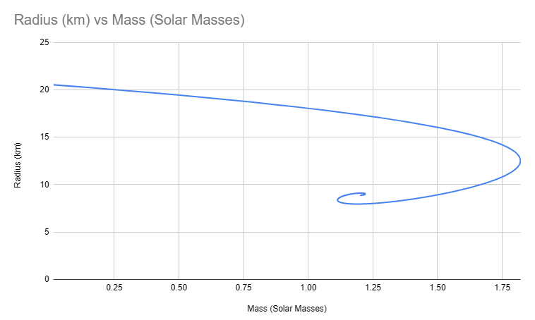
This means that there might be multiple solutions for the central density for a specific ADM mass, and for realistic neutron stars there are at least two. Which makes this problem much more annoying. Anyway, lets write a basic procedure for this:
//personally i liked the voyage home better
std::vector<double> tov::search_for_adm_mass(double mass, const tov::eos::base& param)
{
    double rmin = 1e-6;
    double min_density = 0.f;
    double max_density = 0.1f;

    std::vector<double> densities;
    std::vector<std::optional<double>> masses;

    int to_check = 200;
    densities.resize(to_check);
    masses.resize(to_check);

    for(int i=0; i < to_check; i++)
    {
        double frac = (double)i / to_check;

        double test_density = mix(min_density, max_density, frac);

        integration_state next_st = make_integration_state(test_density, rmin, param);
        std::optional<integration_solution> next_sol_opt = solve_tov(next_st, param, rmin, 0.);

        std::optional<double> mass;

        if(next_sol_opt)
            mass = next_sol_opt->M_msol;

        densities[i] = test_density;
        masses[i] = mass;
    }

    std::vector<double> out;

    for(int i=0; i < to_check - 1; i++)
    {
        if(!masses[i].has_value())
            continue;

        if(!masses[i+1].has_value())
            continue;

        double current = masses[i].value();
        double next = masses[i+1].value();

        double min_mass = std::min(current, next);
        double max_mass = std::max(current, next);

        if(mass >= min_mass && mass < max_mass)
        {
            auto get_mass = [&](double density_in){
                integration_state st = make_integration_state(density_in, rmin, param);
                integration_solution next_sol = solve_tov(st, param, rmin, 0.).value();

                return next_sol.M_msol;
            };

            double refined = tov::invert(get_mass, mass, densities[i], densities[i + 1], false);

            out.push_back(refined);
        }
    }

    return out;
}
This is a two step bruteforcer: First, I do a rough stepping over the parameter space, and then once I’ve found candidate central densities, I perform a high precision bruteforce via the invert function. This likely fails right at the vertical cusps of the neutron star graphs, but it works well in general
The lower density branch here (with larger radius) is the correct neutron star in our case if we’re looking for test case C1, which we simply have to know a-priori
TOV: Mass vs rest mass, and calculating the rest mass $M_0$
The $M$ we’ve calculated corresponds to ADM mass - sometimes called gravitational/gravitating mass. It is the mass as measured as a gravitational field
The rest mass $M_0$ is the integral of the rest-mass density, over the volume of the neutron star. These aren’t the same, as due to the self warping of space by a neutron star, more matter can fit into its volume than you’d expect
This next section is often left a bit underspecified, so here it is in detail: In GR, if you want to integrate something, you have to integrate it multiplied by the volume element. In GR, this is $\sqrt{\mid \mathrm{det}\; g \mid}$, where $g$ is the metric. This measures the volume of a parallelpiped, with dimensions $dx^0 dx^1 dx^2 dx^3$. However, we only actually want the volume element in the $r$ direction as we’re integrating if we want to calculate the rest mass, which is $\sqrt{\mid(1 - 2\frac{m}{r})^{-1}\mid}$, or $(1 - 2\frac{m}{r})^{-\frac{1}{2}}$ here. This is how wikipedia gets its equation for gravitational binding energy
So, to calculate $M_0$, we can do this:
\[\frac{dM_0}{dr} = 4 \pi \rho_0 r^2 (1 - 2\frac{m}{r})^{-\frac{1}{2}}\]This is the rest mass density integrated over the volume of the neutron star
Often, you see a similar equation of the following form, which is what wikipedia has:
\[\frac{dEnergy}{dr} = 4 \pi \mu r^2 (1 - 2\frac{m}{r})^{-\frac{1}{2}}\]This is the energy stored within the neutron star
Armed with this information, we can calculate $M_0$ in this paper for their different values, and realise that they’ve mixed up ADM mass and rest mass in many places. This seems to be a common mistake, and there is often an implicit conversion between the two that I’m not convinced everyone actually does. I myself was caught out by this until I started adding more test cases, and realised that I’d made seemingly the exact same error hilariously. As always, literature replication is a disaster, and I’m perpetually figuring new things out
ADM formalism conversions
| Symbol | Name | Relation to normal GR | Description |
|---|---|---|---|
| $\gamma_{ij}$ | The 3-metric tensor | $g_{ij}$ | Describes curvature on the 3 surface. Symmetric |
| $K_{ij}$ | Extrinsic curvature | $\frac{1}{2 \alpha} (D_i \beta_j + D_j \beta_i - \frac{\partial g_{ij}}{\partial_t})$ | The curvature of the 3 surface with respect to the 4th dimension. Symmetric. Note that $\frac{\partial g_{ij}}{\partial_t} = \frac{\partial \gamma_{ij}}{\partial_t}$ |
| $\alpha$ | Lapse | $\sqrt{-g_{00} + \beta^m \beta_m}$ | Part of the hypersurface normal, which points into the future |
| $\beta^i$ | Shift | $g_{0i}$ | The other part of the hypersurface normal, which points into the future |
BSSN formalism conversions
| Symbol | Name | Relation to ADM | Notes |
|---|---|---|---|
| $W$ | Conformal factor | $det(\gamma_{ij})^{-\frac{1}{6}}$ | Describes the relationship between the ADM variables, and the conformal BSSN variables. $W=0$ at a singularity |
| $\tilde{\gamma}_{ij} $ | Conformal metric tensor | $W^2 \gamma_{ij}$ | Raises and lowers the indices of conformal variables. Inverted as if it were a 3x3 matrix. Symmetric, and has a unit determinant |
| $K$ | Trace of the extrinsic curvature | $\gamma^{ij} K_{ij}$ | |
| $\tilde{A}_{ij}$ | Conformal extrinsic curvature | $W^2 (K_{ij} - \frac{1}{3} \gamma_{ij} K)$ | Trace free, symmetric |
| $\tilde{\Gamma}^i$ | Conformal Christoffel symbol | $\tilde{\gamma}^{jk} \tilde{\Gamma}^i_{jk}$ | Evolved numerically despite having an analytic value from conformal variables, for stability reasons |
| $\alpha$ | Lapse | $\alpha$ | No change |
| $\beta^i$ | Shift | $\beta^i$ | No change |
$W$, aka the Lorentz factor, extended discussion
This is the segment of the paper where things start to get a tad wonky. If we skip to the initial data procedure, we can see that just after (66), it says:
“In this equation, the boost factor W for the stellar model is given by Eq. (60) for linear momentum or Eq. (65) for angular momentum”
Given that the language is identical to the language used for $\bar{A}_{ij}$, a casual read of this might suggest one of the two following things:
- We sum the Lorentz factors22
- We sum the quantity $\left [(\bar{\mu} + \bar{p}) W^2_{type} - \bar{p} \right ]$ for the angular, and linear Lorentz factors
These two Lorentz factors are given as follows:
Linear (60):
\[W_{P}^2 = \frac{1}{2}\left (1 + \sqrt{1 + \frac{4 P_i P^i}{\mathcal{M}^2}} \right)\]Angular (65):
\[\begin{align} W_{J}^2 &=\frac{1}{2}\left (1 + \sqrt{1 + \frac{4 J_i J^i r^2 \sin^2 \theta}{\mathcal{N}^2}} \right)\\ \sin^2 \theta &= 1 - (\hat{J}^i \hat{l}_i)^2 \\ \end{align}\]$l_i$ is the same unit normal as earlier. For $\sin^2 \theta$, $J^i$ and $l_i$ are normalised (hence the hats) to a length of $1$, as I’ve plugged in the formula $\mathrm{dot}(a, b) = \cos \theta \mid a\mid \;\mid b\mid $. $\theta$ more technically is the angle between $J^i$ and $l^i$. Note that the quantity $\theta$ becomes undefined as $J^i J_i$ tends to $0$, but given the prefix term, $\sin^2 \theta$ can be set to anything when this happens
Now. The tricky part comes in in that both of these options can be straightforwardly shown to be incorrect. See, a Lorentz factor is $1$ when it corresponds to no velocity. This means that if we trial setting $W=1$ for both contributions to run a basic sanity check for this procedure, our summed Lorentz factor is:
\[W_{sum} = W_J + W_P = 2\]Which isn’t right, as a stationary fluid should have a Lorentz factor of $1$. Running the same idea for superimposing the matter terms gives a similar answer:
\[\bar{\mu}_H^{summed} = ((\bar{\mu} + \bar{p}) W^2_P - \bar{p}) + ((\bar{\mu} + \bar{p}) W^2_J - \bar{p}) = 2 \bar{\mu}\]Which is also clearly incorrect - we really can’t just sum things that have a Lorentz factor in them, as it doesn’t add linearly. This paper, other (e1), (e2) papers by the same authors referencing this procedure, and the thesis on which this paper is based do not specify the details on how this works. This paper does construct a neutron binary with spinning and moving neutron stars, so its clear that its being done somehow (figure 8a clearly has linear momentum, and its a spinning test case), it just does not specify how
You might consider that we could add Lorentz factors via a rapidity formula, but this is incorrect as these two terms are Lorentz factors representing velocities in a direction
Searching slightly further afield
Now, that’s not the only definition of the Lorentz factor in this paper. We also have (27):
\[W^2 = \frac{1}{2}\left [1 + \sqrt{1 + \frac{4 \bar{\gamma}_{ij} \bar{S}^i \bar{S}^j}{(\bar{\mu} + \bar{p})^2}}\right]\]Which brings up the question: What’s $\bar{S}^i$? Well, we have two quantities here, defined via (32) and (33):
\[\begin{align} \bar{S}^i &= P^i \sigma(r) \\ \bar{S}_i &= \epsilon_{ijk} J^j x^k \kappa(r) \end{align}\]The question becomes, can we just add these together (after raising the second quantity), or do we have to do something more complex like calculating the 4-velocities and doing Lorentz boosts? Off-hand, its tricky to know what to do with it
This is a bit odd
This is a strange one - the procedure laid out here is incomplete unfortunately. After the maximal slicing and conformal flatness assumption, we end up with the relation:
\[\bar{\nabla}_j \bar{A}^{ij} = 8 \pi \bar{S}^i\]Which here simplifies to $\partial_j \bar{A}^{ij} = 8 \pi \bar{S}^i$. This is a very chopped down form of the momentum constraint. Solutions to this equation are linear, so we can take the sum of the two $\bar{A}^{ij}$’s calculated earlier for a single star, and use that to derive $\bar{S}^i$. Then derive the Lorentz factor from its equation up above (27)
Its likely that this also implies that we can sum the individual sources $\bar{S}^i$. Ie, because of the linearity, we can say:
\[\bar{\nabla}_j \bar{A}^{ij}_J + \bar{\nabla}_j \bar{A}^{ij}_P = 8 \pi \bar{S}_J^i + 8 \pi \bar{S}_P^i\]Which further implies that $S_{new}^i = S_J^i + S_P^i$. It seems correct enough
In general, this kind of step being left out of a paper can consume a significant amount of investigatory time unfortunately, but it comes with the territory, and literature replication is always difficult23
Unnecessary further investigation
After writing this all, I decided to reach out to the author, which is something I never do - but I’m loathe to present speculation here. They said two things:
- They state they have not done neutron stars with both spin and linear momentum
- If you want both, you should add the two $\bar{S}^i$ components together, and calculate the Lorentz factor from (27)
I’m going to leave this topic alone now, this segment was really just to illustrate some of the joy that goes into this
Useful References/Further reading
I only discovered this after I’d implemented everything, but it looks like a good resource:
https://github.com/zachetienne/nrpytutorial/blob/master/Tutorial-ADM_Initial_Data-TOV.ipynb
Primary TOV reference https://einsteintoolkit.org/thornguide/EinsteinInitialData/TOVSolver/documentation.html
Primary paper reference for the second half of this article https://arxiv.org/pdf/1606.04881
Hydrodynamics papers used:
https://arxiv.org/pdf/gr-qc/9908027
https://arxiv.org/pdf/gr-qc/0209102
Unit conversions: https://www.seas.upenn.edu/~amyers/NaturalUnits.pdf
Useful TOV reference: https://www.as.utexas.edu/astronomy/education/spring13/bromm/secure/TOC_Supplement.pdf
Relativistic radiative transfer equations for raytracing: https://arxiv.org/pdf/1207.4234. There may or may not be an article about implementing this. A basic version of these equations has been included
-
My email is icedshot@gmail.com, or if you’d like - follow my bluesky at @spacejames.bsky.social. Please feel free to contact me for any reason at all, even if you want to just chit chat or nerd out about space ↩
-
Everything in this article could also be used to describe less crazy stars or planets, which would have correspondingly different equations of state ↩
-
I believe that strictly speaking the equation of state only necessarily relates the energy of matter to the pressure, but in this article I’m going to assume we can convert between energy, density, and pressure freely ↩
-
You can think of the ADM mass as being the ‘gravitational’ mass, and the rest mass as being the amount of matter ↩
-
They’re structured in a form to compare with newtonian theory, as a post newtonian analysis. They are however not super useful ↩
-
This is one of the areas of the literature where the notation is unfortunately very muddled, so I’m going to try very hard to be as consistent as humanly possible. ↩
-
I’m not incredibly sure about this. I’ve calculated this to make the units pan out between $\mu$ and $\rho_0$ via $\mu = \rho_0 (1 + \epsilon)$. If this is wrong, please let me know. You never actually need to do unit conversions on this variable, but still it’d be nice to be correct here ↩
-
yep ↩
-
The actual mass of the sun would be a terrible idea to use, given that it varies and has error bars. So the mass of the sun is a defined constant which is nearly equivalent ↩
-
I’ve seen multiple reports in the literature that these equations are very stiff and hard to solve, but have not found this in practice ↩
-
If you’d like a peek behind the scenes on the development of these articles, it took me several days and 1k+ lines of code to figure out that this was the error that was preventing my integrator from working properly. One of the reasons why I’m being as pedantic as possible about units, and coordinate systems, is to try and help other people avoid my mistakes ↩
-
My biggest conspiracy theory is that this is because K, without the K, is pronounced A. This is almost definitely wrong, but its much more fun to believe ↩
-
Note that I think this paper implicitly assumes that $n = (1, 0, 0, 0)$. Ie $\alpha = 1$, $\beta^i = 0$. This doesn’t affect the lapse or shift we can set later, as its essentially an implementation detail, but this will crop up in the next article when we initialise our hydro variables ↩
-
I’m trying to stem some of the incredibly random notational divergence in the literature. This area has extremely inconsistent notation ↩
-
I explicitly picked this paper because it allows us to construct multiple black holes and neutron stars together ↩
-
It uses what I personally think is one of the most interesting results in GR: Any spherically symmetric vacuum spacetime is locally the Schwarzschild metric. So exterior to our star in the stationary solution, it matches a Schwarzschild solution with some mass, to the tov solution so they line up correctly ↩
-
https://physics.stackexchange.com/questions/145342/schwarzschild-metric-in-isotropic-coordinates ↩
-
You might also find yourself wanting to use dimensionless spin: $\chi = \frac{J}{M^2}$ ↩
-
When I first read this paper many years ago, I had virtually no physics background, and nearly all my maths experience was related to 3D graphics. It is fair to say that I was not the target market for this paper. You can probably see a few remnants in this article of other basic mistakes I made with the notation back then, by clarifications that I make that are likely super obvious to someone with a physics background ↩
-
I’d still recommend it over writing the equivalent code in OpenCL/CUDA by hand though ↩
-
This only works if the stars are not overlapping ↩
-
Do note that this argument is more for illustrative purposes to demonstrate that the second case is wrong, for a reader who is less able to immediately spot that this is an error. If you’re more familiar with GR, you’ll know that there are other more obvious grounds to rule this out immediately (in that Lorentz factors not adding together is basic GR) ↩
-
In general, its clear that the procedure implemented is not entirely the one described. In this paper (82) is incorrect. In this paper, the mistake is repeated as (31). In a later paper, this mistake is corrected as (22) ↩